This work is licensed under a Creative Commons Attribution-NonCommercial-ShareAlike 4.0 International License. Exceptions to this license are the Figures 3.2, 3.3, 3.5, 3.15 and 8.4. Permission is granted to reproduce these figures as part of this work in both print and electronic formats, for distribution worldwide in the English language. All other copyrights for Figures 3.2, 3.3, 3.5, 3.15 and 8.4 belong to their respective owners. Links are provided throughout the text to Wikipedia articles, which are released under the Creative Commons Attribution-Share-Alike License 3.0.
This derivative work is authored by Rico A.R. Picone from the original by Professors Francesco Bullo and Stephen L. Smith. The author is grateful to Professors Bullo and Smith for their willingness to share their work and allow it to be remixed. The original was Version v0.92(b) (9 Mar 2021). For the latest original version, see motion.me.ucsb.edu/book-lrpk.
Preface
Topics
These undergraduate level lecture notes cover motion planning and kinematics with an emphasis on geometric reasoning, programming and matrix computations. In the context of motion planning, we present sensor-based planning, configuration spaces, decomposition and sampling methods. In the context of kinematics, we present reference frames, rotation matrices and their properties, displacement matrices, and kinematic motion models.
This book is a collection of lecture notes and is not meant to provide a comprehensive treatment of any topic in particular. For more comprehensive textbooks and more advanced research monographs, we refer the reader to a rich growing literature.Murray, Li, and Sastry, A Mathematical Introduction to Robotic Manipulation; Spong, Hutchinson, and Vidyasagar, Robot Modeling and Control; Craig, Introduction to Robotics; Siciliano et al., Robotics; Mason, Mechanics of Robotic Manipulation; Corke, Robotics, Vision and Control; Siegwart, Nourbakhsh, and Scaramuzza, Introduction to Autonomous Mobile Robots; Choset et al., Principles of Robot Motion; LaValle, Planning Algorithms; Selig, Geometrical Methods in Robotics; Thrun, Burgard, and Fox, Probabilistic Robotics; Dudek and Jenkin, Computational Principles of Mobile Robotics; Jazar, Theory of Applied Robotics; Niku, Introduction to Robotics; Kelly, Mobile Robotics.
The intended audience and use of these lectures
These lecture notes are intended for undergraduate students pursuing a 4-year degree in mechanical, electrical or related engineering disciplines. Computer Science students will find that the chapters on motion planning overlap with their courses on data structures and algorithms. Prerequisites for these lecture notes include a course on programming, a basic course on linear algebra and matrix theory, and basic knowledge of ordinary differential equations.
These lecture notes are intended for use in a course with approximately 30-36 contact hours (e.g., roughly one chapter per week in a 10-week long course). Student homework includes standard textbook exercises as well as an extensive set of programming exercises (focused on motion planning). We envision this textbook to be used with weekly homework assignments, weekly computer laboratory assignments, a midterm exam, and a final exam.
For the benefit of instructors, these lecture notes are supplemented by two documents. First, a solutions manual, including programming solutions, is available upon request free of charge to instructors at accredited institutions. Second, these lecture notes are also available in “slide/landscape” format especially suited for classroom teaching with projectors or screens.
Learning Objectives
Course learning outcomes, i.e., skills that students should possess at the end of a 10-week course based upon these lectures, include:
an ability to apply knowledge of geometry, graph algorithms, and linear algebra to robotic systems,
an ability to use a numerical computing and programming environment to solve engineering problems,
an ability to formulate, and solve motion planning problems in robotics, and
an ability to formulate and solve kinematics problems in robotics.
Implementation via Programming
These notes contain numerous algorithms written in pseudocode and numerous programming assignments. We ask the reader to choose a programming language and environment capable of numerical computation and graphical visualization. Typical choices may be Matlab and Python (with its packages numpy and scipy). Later programming assignments depend upon earlier ones and so readers are advised to complete the programming assignments in the order in which they appear.
Readers should be informed that the purpose of the programming assignments is to develop their understanding of algorithms and their programming ability. For more advanced purposes (e.g., commercial enterprises or research projects), we refer to CGAL for an efficient and reliable algorithm library available as open source software; see Fabri and Pion“CGAL:The Computational Geometry Algorithms Library.”
or The CGAL Project,CGAL User and Reference Manual.
and to the “The Motion Strategy Library” and the “Open Motion Planning Library” for motion planning libraries by LaValle and others“The Motion Strategy Library.”
and Şucan, Moll, and Kavraki,“The Open Motion Planning Library.”
respectively.
Acknowledgments
First, we wish to thank Joey W. Durham, who designed and implemented the first version of many exercises and programming assignments, and Patrick Therrien, who prepared a comprehensive set of programming solutions in Matlab and Python. We are also very thankful to all instructors who were early adopters of these lecture notes and provided useful feedback, including Professors Sonia Martı́nez and Fabio Pasqualetti. Finally, it is our pleasure to thank Anahita Mirtabatabaei, Rush Patel, Giulia Piovan, Cenk Oguz Saglam, Sepehr Seifi and Carlos Torres for having contributed in various ways to the material in these notes and in the assignments.
1 Sensor-based Planning
Introduction
In this chapter we begin our investigation into motion planning problems for . We consider the fundamental robotic task of moving from a starting point \(A\) to goal point \(B\) in an environment with obstacles. This chapter focuses on sensor-based motion planning, where the obstacles are initially unknown to the robot, and the robot acquires information about its surroundings using onboard sensors as it moves. Whether or not a robot can succeed at navigating from start to goal will depend on its sensors and capabilities. In this chapter we
introduce three bug algorithms for sensor-based motion planning,
define notions of and for motion planning algorithms, and
study the completeness of the three bug algorithms.
1.1 Problem setup and modeling assumptions
Motion planning is an important and common problem in robotics. In its simplest form, the motion planning problem is: how to move a robot from a “start” location to a “goal” location . This problem is sometimes referred to as the “move from A to B” or the “piano movers problem” (how do you move a complex object like a piano in an environment with lots of obstacles, like a house).
In this first chapter, we consider a sensor-based planning problem for a point moving in the plane \(\real^2\). In other words, we assume the robot has a sensor and, based on the sensor measurements, it plans its motion from start to goal. To properly describe the motion planning problem, we need to specify: what does the robot have? What does the robot have?
In this chapter, we make the following assumptions on the robot and its environment. As illustrated in fig. 1.1, we are given
a workspace \(W\) that is a subset of \(\real^{2}\) or \(\real^{3}\), often just a rectangle;
some obstacles \(O_{1}, O_{2},\ldots,O_n\);
a start point \(\subscr{p}{start}\) and a goal point \(\subscr{p}{goal}\); and
a robot described by a moving point (that is, the robot has zero size).
Figure 1.1: The environment for sensor-based planning
We define the \(\subscr{W}{free} = W \setminus (O_1 \union O_2 \union \cdots \union O_n)\) as the set of points in \(W\) that are outside all obstacles. (Recall the definition of the set \(A\setminus B = \setdef{a\in A}{a\not\in B}\), that is, all points in \(A\) that are not in \(B\).)
Robot Assumptions
We also make some assumptions on the capabilities and knowledge of the robot. We assume the robot:
knows the direction towards the goal,
knows the straight-line distance between itself and the goal,
does not know anything about the obstacles (number, location, shape, etc),
has a contact sensor that allows it to locally detect obstacles,
can move either in a straight line towards the goal or can follow an obstacle boundary (possibly by using its contact sensor), and
has limited memory in which it can store distances and angles.
We discuss in more detail later what these robot capabilities imply in terms of robot sensors and knowledge.
Our task is to plan the robot motion from the start point to the goal point. This plan is not a precomputed sequence of steps to be executed, but rather a policy to deal with the possible obstacles that the robot may encounter along the way.
Environment Assumptions
Finally, we make some assumptions on the workspace and obstacles:
the workspace is ,
there are only a finite number of obstacles,
the start and goal points are in the free workspace \(\subscr{W}{free}\), and
any straight line drawn in the environment crosses the boundary of each obstacle only a finite number of times. (This assumption is easily satisfied for “normal objects” and we will use it later on to establish the correctness of our algorithms.)
In the next sections we see three different algorithms for planning the robot motion from start to goal, called Bug 0, Bug 1, and Bug 2. Each algorithm has slightly different requirements on the robot’s capabilities and knowledge. As a result, we will also see that they have different in finding paths from start to goal.
1.2 The Bug 0 algorithm
Starting from the scenario illustrated in fig. 1.1, suppose the robot heads towards the goal position from the start position. How does the robot handle with obstacles? (Note that the robot sensor is local so that the robot only knows it has hit an obstacle.) We need a strategy to avoid the obstacle and move towards the goal destination.
What follows is our first motion planning algorithm.
Bug 0 algorithm
Moving to the left means that the robot is just sliding along the obstacle boundary, i.e., circumnavigating the obstacle boundary in a clockwise fashion. The moving direction, left or right, is fixed but irrelevant. We only need to designate one preferred direction to turn once the robot hits an obstacle. A right-turning robot will circumnavigate an obstacle in a counterclockwise fashion. A right-turning robot follows the same path as a left-turning robot in a reflected world.
As shown in fig. 1.2 we label the point on the obstacle boundary where the robot hits the obstacle as \(\subscr{p}{hit}\) and the point on the obstacle boundary where the robot leaves as \(\subscr{p}{leave}\).
Figure 1.2: A successful execution of the Bug 0 algorithm
Note: we are not being very careful clarifying whether the robot moves in or in . For now imagine that the robot can move smoothly, visit all boundary points, take a measurement at each point and store the distance from the closest boundary point.
The Bug 0 algorithm does not always find a path to the goal
Unfortunately, our Bug 0 algorithm does not work properly in the sense that there are situations (workspaces, obstacles, start and goal positions) for which there exists a solution (a path from start to goal) but the Bug 0 Algorithm does not find it. We will talk more later about the correctness of an algorithm and in particular about the notion of .
This example in the fig. 1.3 illustrates a periodic loop generated by the Algorithm Bug 0. At the end of each loop there is no complete progress to goal.
Figure 1.3: An unsuccessful execution of the Bug 0 Algorithm
1.3 The Bug 1 algorithm
The fact that Bug 0 does not always find a path to the goal may not be too surprising: The algorithm is not making use of all of the capabilities of the robot. In particular, the algorithm does not use any , nor does it use the distance to the goal. This observation motivates our second smarter sensor-based algorithm for a more capable bug.
Bug 1 algorithm
a
b
Figure 1.4: Two successful executions of the Bug 1 Algorithm.
Note: the only difference between Bug 0 and Bug 1 is the reaction to the obstacle encounter, i.e., the behavior inside the if command.
1.3.1 Implementing Bug 1
The Bug 1 algorithm can be implemented as follows. In the simplest version, when the robot hits an obstacle at \(\subscr{p}{hit}\), it records the distance and direction to the goal. The robot then circumnavigates the obstacle, storing in memory a variable containing the minimum distance from its current position along the obstacle boundary to the goal. Regarding instruction 4, the circumnavigation is complete when the robot returns to the distance and direction it recorded at \(\subscr{p}{hit}\). The robot then circumnavigates the obstacle a second time until its distance to goal matches the minimum distance it has stored in memory.
In a more sophisticated version, the robot would additionally measure the distance it travels while circumnavigating the obstacle and therefore return to the closest point along the boundary using the of the clockwise and counterclockwise paths. An instrument for measuring distance traveled is known as a linear odometer. If the robot moves at constant speed, then a clock suffices as a linear odometer: distance traveled is equal to speed times travel time. If the robot’s speed is variable, then one typically uses encoders in the robot wheels to measure the number of wheel rotations.
In summary, the Bug 1 robot must have memory for storing information about \(\subscr{p}{hit}\) and for computing \(\subscr{p}{leave}\) and it benefits from (but does not require) a linear odometer, i.e., an instrument to measure traveled distance.
1.3.2 Flowcharts
Before we proceed any further, it is useful to stop and discuss how to represent algorithms. So far we have adopted the representation, i.e., a simplified English-like language that is midway between English and computer programming. It is also useful to understand how to represent our algorithms using flowcharts. Since flowchart representations can become quite large, they are typically useful for only simple programs.
According to Wikipedia:pseudocode, “pseudocode is compact and informal high-level description of a computer programming algorithm that uses the structural conventions of a programming language, but is intended for human reading rather than machine reading.”
According to Wikipedia:flowchart, “a flowchart is a type of diagram that represents an algorithm or process, showing the steps as boxes of various kinds, and their order by connecting these with arrows.”
The four constitutive elements of a flowchart
A flowchart consists of four symbols shown in fig. 1.5, which can be thought of as a graphical language.
a
b
c
d
Figure 1.5: The four elements of a flowchart. a — Circles represent the start and terminating point, b — Arrows indicate the flow of control, c — Rectangles represent a single command, d — Diamonds output 2 paths based on a binary question
Note: The dominant convention in drawing flowcharts is to have the flow of control go from and .
1.3.3 Flowchart representation for the Bug 1 Algorithm
Figure 1.6: Flowchart representation for the Bug 1 Algorithm
If you examine carefully the Bug 1 flowchart of fig. 1.6, you can clearly see that the algorithm may end in failure. This is indeed possible if the workspace is composed of disconnected components (that is, pieces of the free workspace that can not be connected with a path), and the start and goal locations belong to distinct disconnected components as shown in fig. 1.7.
Figure 1.7: Environment for which no path exists from start to goal
1.3.4 The performance of the Bug 1 algorithm
Next, let us begin to rigorously analyze the Bug 1 algorithm. There are 2 desirable properties we wish to establish:
(with respect to some desirable metric), and
(i.e., correctness in an appropriate sense).
We begin with the simpler analysis, i.e., the study of optimality. We are interested in seeing how efficient is the algorithm in completing its task in a workspace with arbitrary obstacles.
The question is: what is the length of the path generated by the Bug 1 Algorithm in going from start to goal? While a precise answer is hard to obtain in general, we can ask three more specific questions:
Will Bug 1 find the path from start to goal?
How long will the path found by Bug 1 be? Can we find a lower bound and an upper bound on the path length generated by Bug 1?
Is there a workspace where the upper bound is required?
In order to answer these mathematical questions, it is good to have some notation: \[\begin{aligned}
D &= \text{length of straight segment from start to goal}, \\
\perim(O_i) &= \text{length of perimeter of the $i$th obstacle}.\end{aligned}\]
[Performance of Bug 1] Consider a workspace with \(n\) obstacles and assume that the Bug 1 algorithm finds a path to the goal. Assuming the robot is not equipped with a linear odometer, the following properties hold:
Bug 1 does not find the shortest path in general;
the path length generated by Bug 1 is lower bounded by \(D\);
the path length generated by Bug 1 is upper bounded by \(D+ 2\sum_{i=1}^n \perim(O_i)\); and
the upper bound is reached in the workspace described in fig. 1.8.
Figure 1.8: An example environment where the upper bound on the performance of Bug 1 is achieved for a robot with a linear odometer.
Note: Assume now that the robot is equipped with a linear odometer. After circumnavigating an obstacle, the robot can therefore move along the of the two paths from hit point to leave point. In this case, the robot will travel at most \(1/2\) of the perimeter to return to the leave point and the upper bound on the path length can be strengthened to \(D+ \frac{3}{2}\sum_{i=1}^n \perim(O_i)\). An example environment achieving this bound is shown on the right of fig. 1.9.
Figure 1.9: An example environment where the upper bound on the performance of Bug 1 is achieved for a robot with a linear odometer.
1.4 The Bug 2 algorithm
Let us now try to design a new algorithm that generates shorter paths than Bug 1. The perceived problem with Bug 1 is that each obstacle needs to be before the robot can proceed towards the goal. Can we do better, i.e., can we decide to leave the obstacle without traversing all its boundary?
We use the term start-goal line to refer to the unique line that passes through the start point and goal point. The start-goal line is the dashed line intersecting the two obstacles as shown on the left of fig. 1.10. To aid in the design of Bug 2, we begin with a preliminary version.
Figure 1.10: The start-goal line, a successful execution of the Bug2.prelim algorithm, and an unsuccessful execution of the Bug 2.prelim algorithm
Bug 2.prelim algorithm
The example execution on the right of fig. 1.10 amounts to an undesired periodic cyclic trap again. How do we improve and possibly fix this misbehavior in our algorithm? It turns out that a small fix is sufficient. For convenience we repeat the entire algorithm, but the only difference is the addition of the requirement that the leave point be than the hit point!
Bug 2 algorithm
From the left of fig. 1.11 we see that Bug 2 finds a path to the goal where Bug 2.prelim did not. Let us briefly mention the requirements of Bug 2, although we will compare them more carefully in sec. 1.4.3. For Bug 0, we assumed the robot can sense direction towards the goal, and it knows when it has reached the goal. For Bug 1 and 2, we assumed the robot can measure and store in memory the distances and directions to goal point that it senses along the boundary. In particular, Bug 2 stores distance and direction at the hit point and compares these two quantities with the ones it senses along the boundary.
1.4.1 Monotonic performance and its implications
Here we briefly discuss why our correction to the Bug 2.prelim algorithm is indeed helpful and has a chance to render the algorithm correct. Consider the function of time equal to the distance between the robot and the goal point (this distance is a function of time because the robot is moving). Let us plot this distance function of time along the execution of the Bug 2 algorithm.
a
b
Figure 1.11: The monotonic performance of Bug 2.
As fig. 1.11 illustrates, the leave point \(\subscr{p}{leave}\) is closer to the goal than the hit point \(\subscr{p}{hit}\). Of course, throughout the search phase (while the robot is moving along the boundary to find the optimal leave point) the distance function may not always decrease, but after the search phase is complete, the robot will indeed be closer to the goal.
This discussion establishes that the distance between the robot and the goal is a function of time, when the robot is away from any obstacles.
Monotonicity immediately implies that there can be no cycles (and therefore no infinite cycles) in the execution of the algorithm. The lack of such cycles is true because (1) the leave point is closer to the goal than the hit point and (2) when the robot moves away from the obstacle the distance continues to decrease. Therefore, it is impossible for the robot to hit the same obstacle again at the same hit point.
1.4.2 The performance of the Bug 2 algorithm
Let us now analyze the performance of the Bug 2 algorithm. With the usual convention (\(D\) is the distance between start and goal and \(\perim(O_i)\) is the perimeter of the \(i\)th obstacle), we have the following results.
[Performance of Bug 2]Consider a workspace with \(n\) obstacles and assume that the Bug 2 algorithm finds a path to the goal. The following properties hold:
Bug 2 does not find the shortest path in general;
the path length generated by Bug 2 is lower bounded by \(D\);
the path length generated by Bug 2 is upper bounded by \[D+ \sum_{i=1}^n c_i \perim(O_i)/2 ,\] where \(c_i\) is the number of intersections of the start-goal line with the boundary of obstacle \(O_i\).
Proof. The first statement is obvious. Regarding the second statement, the lower bound is the same as that for Bug 1 – no surprise here. Regarding the third statement, the upper bound is different from that for Bug 1 and is due to the following fact: each time Bug 2 hits an obstacle (at a hit point), it might need to travel the obstacle’s perimeter before finding an appropriate leave point. So for each pair of hit point and leave point (\(2\) intersection points), the Bug 2 travels at most the obstacle’s perimeter. ◻
1.4.3 Comparison between bug algorithms
After introducing the Bug 1 and Bug 2 algorithms, let us compare in terms of path length. We ignore Bug 0 in this discussion because we already established it is not correct via the example in fig. 1.3. Without losing any generality, let us assume both the Bug 1 and Bug 2 algorithms are left-turning.
Example where Bug 2 finds shorter path than Bug 1
Recall that the Bug 2 algorithm was introduced in an attempt to find paths by not fully exploring the boundary of each encountered obstacle. Indeed it appears that Bug 2 works better in our running example, as shown in fig. 1.12.
a
b
Figure 1.12: Example environment in which Bug 2 is better than Bug 1. a — Bug 1, b — Bug 2
However, it is not clear that this fact must hold true for any problem (remember that a problem is determined by the workspace, the obstacles, and start and goal positions).
Counterexample where instead Bug 1 is better than Bug 2
Looking at the environment in fig. 1.13, we see that Bug 1 explores the entire perimeter of the obstacle only once and then moves to point \(\subscr{p}{leave}\) before leaving the obstacle for the goal. Bug 2, on the other hand, takes a much longer path. Indeed, whenever a robot implementing Bug 2 encounters a “left finger” in the environment, it ends up traveling all the way back near to the start position.
a
b
Figure 1.13: Example environment where Bug 1 is better than Bug 2. Bug 1 has one pair of hit and leave points. Bug 2 hits and then leaves the obstacle four times, as shown by the sequence of hit and leave points.. a — Bug 1, b — Bug 2
Summary of path length
Bug 1 performs an by examining all possible leave points before committing to the optimal choice. Bug 2 is a greedy algorithm that takes the first-available leave point that is closer to the goal without any specific performance guarantee. While it is impossible to predict which of the two will outperform in an arbitrary environment, we may say that Bug 2 will outperform Bug 1 in many simple environments but Bug 1 has more predictable performance.
Summary of robot capabilities
The bug algorithms have slightly different assumptions on the sensors and capabilities needed by the robot.
tbl. 1.1 summarizes these capabilities: direction to goal, distance to goal, memory, linear odometer, and a new capability called an angular odometer or a compass. Recall that a linear odometer was an optional sensor/capability for Bug 1 and it allowed the robot to return to the leave point using the shorter of the two paths along the boundary.
Table 1.1: Summary of the robot capabilities needed to implement each bug algorithm
Sensor/Capability
Bug 0
Bug 1
Bug 2
direction to goal
yes
yes
yes
distance to goal
no
yes
yes
memory
linear odometer
no
optional
no
angular odometer or compass
no
yes
yes
The new sensor/capability of an "angular odometer or compass" is needed in order for the robot to the direction to goal in memory. This is required in Bug 1 to determine when circumnavigation is complete, and in Bug 2 to determine when the start-goal line is encountered. The direction to goal must be stored in a known (for example, as a counterclockwise angle relative to a fixed \(x\)-axis) so that measured directions can be compared to the stored directions. The robot could define a local reference frame based on its heading, but this frame would rotate with the robot. It is not useful to store a direction in such a frame, unless the robot also somehow records the orientation of the frame when the direction was measured.
There are two possible fixes for this problem, illustrated in fig. 1.14. The first option is that the robot has a compass, and can then record the direction to goal relative to a fixed orientation as given by the compass. This is shown as the angle \(\alpha_1\) relative to north on the left of fig. 1.14. The second option is that the robot can use an angular odometer to measure changes in its heading. The robot can use its initial heading at \(\subscr{p}{start}\) as the orientation for its reference frame. The direction to goal can be specified in this initial frame as the sum of two angles, as shown on the right of fig. 1.14: the angle \(\alpha_2\) can be measured with the aid of an angular odometer, and the angle \(\alpha_3\) is the output of the “direction to goal” sensor.
a
b
Figure 1.14: Bug reference frames. a — The robot records the direction to goal as an angle \(\alpha_1\) relative to north., b — The robot measures the direction to goal as \(\alpha_2 + \alpha_3\), where \(\alpha_2\) must be measured from angular odometer. The angle \(\alpha_3\) is what is given by the “direction to goal” sensor.
This discussion highlights some subtleties in the assumptions we have made on robot capabilities. While the Bug algorithms seem very simple at first glance, they actually require fairly strong assumptions on the sensing and knowledge of the robot. These assumptions are discussed in more detail by Taylor and LaValle.“I-Bug.”
1.5 The completeness of the Bug 1 algorithm
Here we follow up on our previous discussions and formally define the of an algorithm.
An algorithm is complete if, in finite time,
it finds a solution (i.e., a path), if a solution exists, or
it terminates with a failure decision, if no solution exists.
Next, we establish that one of our proposed algorithms is indeed complete. This result was originally obtained by Lumelsky and Stepanov.“Path Planning Strategies for a Point Mobile Automaton Moving Amidst Unknown Obstacles of Arbitrary Shape.”
[Completeness for Bug 1] The Bug 1 algorithm is complete (under the modeling assumptions stated early in the chapter).
1.5.1 On the geometry of closed curves
To prove Theorem 1.4, we start by introducing a wonderful and useful geometric result.
[The Jordan Curve Theorem] Every non-self-intersecting continuous closed curve divides the plane into connected parts. One part is bounded (called the inside) and the other part is unbounded (called the outside) and the curve is the boundary of both parts.
Figure 1.15: A closed curve divides the plane into two parts: the inside and the outside.
Next, consider the following. Imagine that the curve describes the boundary of the obstacle. Given a start and goal point outside the curve (obstacle), connect the two points using a straight segment and count the number of intersections between the segment and the boundary of the obstacle.
It is easy to see that this number of intersections must be (where we regard \(0\) as an even number). Each time the segment enters the inside of the curve, it must then return to the outside. A few examples are given in fig. 1.16.
a
b
c
Figure 1.16: The number of intersections between a line segment and a closed curve, where the endpoints of the segment lie on the outside of the curve, is even.. a — 0 intersections, b — 2 intersections, c — even number of intersections
1.5.2 Proof of the completeness theorem
Here we prove Theorem 1.4. Recall that the Bug 1 algorithm is presented in pseudocode and a flowchart in sec. 1.3.
By contradiction, assume Bug 1 does not find a path, even if a path exists
Let us prove the theorem by . That is, we assume that Bug 1 is incomplete and we find a contradiction. Consider the situation when a path from start to goal does exist, but Bug 1 does not find it. The flowchart description of Bug 1 implies the following statement: if Bug 1 does not find the path, then necessarily Bug 1 will either terminate in failure in finite time or keep cycling forever.
Bug 1 cannot keep cycling forever
Suppose Bug 1 cycles forever. Because there is a finite number of obstacles, the presence of an infinite cycle implies the robot must hit the same obstacle . Now, during the execution of Bug 1, the distance to the goal is a function of time that is monotonically decreasing when the robot is away from any obstacle. Moreover, when the robot hits an obstacle, the distance from \(\subscr{p}{leave}\) to the goal is strictly lower than the distance from \(\subscr{p}{hit}\) to the goal (this fact can be seen geometrically). Therefore, when the robot leaves an obstacle it is closer to the goal than any point on the obstacle. Hence, Bug 1 hit the same obstacle twice.
Bug 1 cannot end in failure, if a path exists
If Bug 1 is incomplete and a path actually exists, then the only possible result is that it terminates in failure. According to the Bug 1 flowchart, failure occurs when: the robot visits all the obstacle boundary points reachable from the hit point, moves to the boundary point \(\subscr{p}{leave}\) closest to the goal, and is unable to move towards the goal. Consider now the segment from \(\subscr{p}{leave}\) to the goal point. Because a path exists from start to goal, a path must also exists between \(\subscr{p}{leave}\) and goal. By the Jordan Curve Theorem, there must be an even number of intersections between this segment and the obstacle boundary. Since \(\subscr{p}{leave}\) is one intersection, there must exist at least another one. Let \(\subscr{p}{other}\) be the intersection point closest to the goal. Now: the point \(\subscr{p}{other}\) has the following properties:
lies on the obstacle boundary,
is reachable from \(\subscr{p}{leave}\) (because it is reachable from the goal), and
is closer to the goal than \(\subscr{p}{leave}\).
These facts are a with the definition of \(\subscr{p}{leave}\).
Figure 1.17: An illustration of the two points \(\subscr{p}{leave}\) and \(\subscr{p}{other}\)
1.6 Appendix: Operations on sets
A set is a collection of objects. For example, using standard conventions, \(\natural\) is the set of natural numbers, \(\real\) is the set of real numbers, and \(\mathbb{C}\) is the set of complex numbers.
If \(a\) is a point in \(A\), we write \(a\in A\). Sets may be defined in one of two alternative ways. A set is defined by either listing the items, e.g., \(A = \{1,2,3\}\), or by describing the items via a condition they satisfy, e.g., \[\begin{aligned}
A &= \setdef{n\in\natural}{n<4}.\end{aligned}\] By convention, the empty set is denoted by \(\emptyset\).
The cardinality of a set \(A\) is the number of elements in \(A\). The set of natural numbers has infinite cardinality. As illustrated in fig. 1.18, the three core set operations are union, intersection, and set-theoretic difference.
a
b
c
Figure 1.18: The three set operations: union, intersection, and set-theoretic difference. a — The union of two sets \(A\) and \(B\) is the collection of points which are in \(A\) or in \(B\) (or in both): \(A \union B = \setdef{x}{x\in A \text{ or } x\in B}\)., b — The intersection of two sets \(A\) and \(B\) is the set that contains all elements of \(A\) that also belong to \(B\): \(A \intersection B = \setdef{x}{x\in A \text{ and } x\in B}\). , c — The set-theoretic difference of two sets \(A\) and \(B\), also known as the relative complement of \(B\) in \(A\) is the set of elements in \(A\) that are not in \(B\): \(A\setminus B = \setdef{a \in A}{a \notin B}\).
A set \(A\) is a subset of \(B\), written \(A \subset B\), if and only if any member of \(A\) is a member of \(B\), that is, \(a \in A\) implies \(a\in B\). Intervals are subsets of the set of real numbers \(\real\) and are denoted as follows: for any \(a<b \in \real\), we define \[\begin{aligned}
{[a,b]} &= \setdef{x}{a\leq{x}\leq{b}}, \\
{]a,b[} &= \setdef{x}{a<x<b}, \\
{]a,b]} &= \setdef{x}{a<x\leq{b}}, \\
{[a,b[} &= \setdef{x}{a\leq{x}<b}.\end{aligned}\] From these interval definitions we have that \({[a,\infty[} = \setdef{x}{a\leq{x}}\), and \({]-\infty,b]} = \setdef{x}{x\leq{b}}\).
The Cartesian product of two sets \(A\) and \(B\) is the set of all possible ordered pairs whose first component is a member of \(A\) and the second component is a member of \(B\): \(A \times B = \setdef{(a,b)}{a \in A \text{ and } b\in B}\). An example is the 2-dimensional plane \(\real^2 = \real \times \real\). We denote the unit circle on the plane by \(\mathbb{S}^1\), the unit sphere in \(\real^3\) by \(\mathbb{S}^2\). We denote the 2-torus by \(\mathbb{T}^2 = \mathbb{S}^1\times \mathbb{S}^1\).
A set \(S \subset \real^d\) is convex if for every pair of points \(p\) and \(q\) within \(S\), every point on the straight line segment that joins them (\(\overline{pq}\)) is also within \(S\): If \(p \in S\) and \(q\in S \Rightarrow \overline{pq} \subset S\), where \(\overline{pq} = \setdef{ \alpha p + (1 - \alpha)q}{\alpha \in [0,1]}\).
Notes and further reading
This chapter is inspired by the original article by Lumelsky and Stepanov,“Path Planning Strategies for a Point Mobile Automaton Moving Amidst Unknown Obstacles of Arbitrary Shape.”
the treatment by Lumelsky,Sensing, Intelligence, Motion.
the first chapter by Choset et al.Principles of Robot Motion.
and the lecture slides by Hager“Algorithms for Sensor-Based Robotics.”
and Dodds.“The Bug Algorithms.”
2 Motion Planning via Decomposition and Search
Introduction
In this chapter we continue our investigation into motion planning problems. As motivation for our interest in planning problems, let us remind the reader that the ultimate goal in robotics is the design of autonomous robots, that is, the design of robots capable of executing without having to be programmed with extremely detailed commands. Moving from \(A\) to \(B\) is one such simple high-level instruction. In this chapter we
study techniques for decomposing the continuous robot workspace into convex regions,
define roadmaps, which encode the decomposed workspace, and
introduce graph algorithms for computing point-to-point paths in roadmaps.
2.1 Problem setup and modeling assumptions
The sensor-based planning problems we studied in the previous chapter are also referred to as closed-loop planning problems in the sense that the robot actions were functions of the robot sensors.This closed-loop type planning is a type of reactive control.
The loop here is the following: the robot moves, then it senses the environment, and then it decides how to move again.
In this chapter we begin our discussion about open-loop planning. By open-loop, as compared with sensor-based and closed-loop, we mean the design of algorithms for robots that do not have sensors, but rather have access to a map of the environment.This open-loop type planning is a type of deliberative control.
Open-loop and closed-loop strategies are synonyms for feedforward and feedback control.
As in the previous chapter, we are given
a workspace that is a subset of \(\real^2\) or \(\real^3\), often just a rectangle,
some obstacles, say \(O_{1},\dots,O_n\),
a start point and a goal point, and
a robot described by a moving point.
As in the previous chapter, we define the free workspace\(\subscr{W}{free}=W\setminus(O_1\union{O_2}\union\cdots\union{O_n})\), see fig. 2.1. We continue to postpone more realistic and complex problems where the robot has a shape, size and orientation.
Figure 2.1: An example free workspace with start and goal locations
Our task is to plan the robot motion from the start point to the goal point via a precomputed open-loop sequence of steps to be executed. We want to design a motion plan under the following modeling assumptions.
Robot Assumptions
The robot has the following capacities:
knows the start and goal locations, and
knows the and .
World Assumptions
The workspace has the following properties:
the workspace is a bounded polygon,
there are only a finite number of obstacles that are polygons inside the workspace, and
the start and goal points are inside the workspace and outside all obstacles.
It is instructive now to compare these new robot and world assumptions with the ones in the previous chapter for sensor-based closed-loop planning. The similarities are the following: (1) the robot is still just a point, it has no size, shape, or orientation, and (2) the robot’s motion is omni-directional (i.e., the robot can move in every possible direction). The differences are the following: (3) the robot has no sensors, but rather knowledge of the free workspace, and (4) planning is now a sequence of pre-computed steps, whereas before sensor-based algorithms are a policy on how to deal with possible obstacles encountered along the way.
2.1.2 Polygons
In these notes, a polygon is a plane figure composed by a finite chain of segments (called sides or edges) closing in a loop. The points where the segments meet are called (or corners). Polygons are always assumed to be simple, i.e., their boundary does not cross itself. Programming-wise, it is convenient to represent a polygon by a counter-clockwise ordered sequence of vertices. (It is our convention not to repeat the first vertex as last.)
As illustrated in fig. 2.1, this chapter assumes that the workspace is a polygon, that each obstacle is a polygon (i.e., a polygonal hole inside the workspace), and that the total number of vertices in workspace and obstacles is \(n\).
2.1.3 Run-time of an algorithm
In this chapter we will study the time it takes for a motion planning algorithm to run, called its run-time, rather than just the length of the path it produces. The run-time of an algorithm is given by the number of computer steps required to execute the code. For the purposes of these notes, we assume that addition, multiplication and division of two numbers can be performed in one computer step. Similarly, we assume a single computer step is required to test if one number is equal to, greater than, or less than another number.
The run-time of an algorithm is a function of the “size” of the input fed to it. If the input has a size \(n\) (for example, the input is a polygon with \(n\) vertices), the runtime is a function \(f(n)\). Counting the exact number of computation steps can be a complex endeavor, and so we instead focus on determining how the run-time scales with \(n\). Rather than saying an algorithm takes exactly \(5n^2 + 4n + 1\) computer steps, it is customary to drop all constants and all lower-order terms, and simply report the run-time as \(O(n^2)\). Formally, the notation is defined as follows.
Given two positive functions \(f(n)\) and \(g(n)\) of the natural numbers \(n\), we write \(f \in O(g)\), if there exist a number \(n_0\) and a positive constant \(K\) such that \(f(n) \le K g(n)\) for all \(n \ge n_0\).
Intuitively, if \(f \in O(g)\), then we are saying that the function \(f\) is less than or equal to the function \(g\) (up to a multiplicative constant and for large \(n\)). In other words, when \(n\) gets large, \(g\) grows at least as fast as \(f\). For example, in fig. 2.2 the function \(f(n)\) grows linearly with \(n\) and \(g(n)\) grows with the square of \(n\), and we have \(f\in O(g)\).
Figure 2.2: The function \(f(n)\) grows linearly with \(n\). The function \(g(n)\) grows with the square of \(n\).
2.2 Workspace decomposition
Introduction
We start with two useful geometric ideas.
Convexity
As mentioned in sec. 1.6, a set \(S\) is convex if for any two points \(p\) and \(q\) in \(S\), the entire segment \(\segment{pq}\) is also contained in \(S\). Examples of convex and non-convex sets are drawn in fig. 2.3. (Here we assume that the set \(S\) is a subset of the Euclidean space \(\real^d\) in some arbitrary dimension \(d\).) For polygons, convexity is related to the at each vertex of the polygon (each vertex of a polygon has an interior and an exterior angle): a polygonal set is convex if and only if each vertex is convex, i.e., it has an interior angle less than \(\pi\). A vertex is instead called non-convex if its interior angle is larger than \(\pi\).
a
b
Figure 2.3: Examples of convex and non-convex sets. A convex set cannot have any hole. Polygons have convex and non-convex interior angles.. a — general set convexity, b — polygonal set convexity
Planning in non-convex sets via convex decompositions
Let us now use the notion of convexity for planning purposes. If the start point and the goal point belong to the same convex set, then the segment connecting the two points is an obstacle-free path. If, instead, the free workspace is not convex, then the following figure and algorithmic ideas provide a simple effective answer.
2.2.2 Decomposition into convex subsets
For complex non-convex environments, we use an algorithm to decompose the free workspace into the union of convex subsets, such as triangles, convex quadrilaterals or trapezoids (quadrilaterals with at least one pair of parallel sides). The following nomenclature is convenient:
the triangulation of a polygon is the decomposition of the polygon into a collection of triangles, and
the trapezoidation of a polygon is the decomposition of the polygon into a collection of trapezoids. (We allow some trapezoids to have a side of zero length and therefore be triangles.)
a
b
Figure 2.4: Planning through a non-convex environment by moving from a convex subset to another. a — Planning through a non-convex environment by moving from a convex subset to another, b — Planning through a non-convex environment by moving from a convex subset to another
It is easy to see that a polygon can be in multiple ways (e.g., consider the two possible diagonals of a square). In what follows we present an algorithm to trapezoidate, i.e., decompose into trapezoids, a polygon with polygonal holes.
sweeping trapezoidation algorithm
The algorithm is among a class of algorithms studied in computational geometry; feel free to inform yourself about this topic at Wikipedia:computational geometry. An execution of the algorithm is illustrated in the fig. 2.5. Note that trapezoids \(T_3\) and \(T_7\) are degenerate, i.e., they are triangles.
a
b
Figure 2.5: A trapezoidation of a workspace into trapezoids \(T_1,\dots,T_{10}\), computed by the sweeping trapezoidation algorithm.
2.2.3 The sweeping trapezoidation algorithm
To understand in more detail how the sweeping trapezoidation algorithm is implemented, consider a workspace in which the boundary is an axis-aligned rectangle and every obstacle vertex has a unique \(x\)-coordinate, i.e., no obstacle segment is vertical. As an example, see fig. 2.5. Since all \(x\)-coordinates are unique, each line segment \(s_i\) describing an obstacle boundary has a left endpoint\(\ell_i\) and a right endpoint\(r_i\), where the \(x\)-coordinate of the left endpoint is smaller than that of the right endpoint. We write this segment as \(s_i = [\ell_i, r_i]\).
To visualize the order in which vertices are processed by the algorithm in step 3, we define a sweeping vertical line \(L\) moving from left to right. Recall, each environment vertex connects line segments. When the line \(L\) hits an environment vertex, we categorize it into one of six types (see fig. 2.6) as summarized in Table tbl. 2.1.
Table 2.1: The six vertex types encountered during the trapezoidal decomposition algorithm
Vertex Type
Vertex as Endpoint of Two Segments
Vertex as Convex or Non-Convex
Example
i
left/left
convex
\(p_6\) and \(p_8\)
ii
left/left
non-convex
\(p_3\)
iii
right/right
convex
\(p_2\) and \(p_4\)
iv
right/right
non-convex
\(p_7\)
v
left/right
convex
\(p_1\)
vi
left/right
non-convex
\(p_5\)
a
b
Figure 2.6: The line segments \(s_1,\dots,s_{10}\) and the obstacle vertices \(p_1,\dots,p_8\) required by the algorithm.
To execute steps 4 and 5 of the sweeping trapezoidation algorithm, we maintain a list \(\mS\) of the obstacle segments intersected by the sweeping line \(L\). The obstacle segments are stored in decreasing order of their \(y\)-coordinates at the intersection point with \(L\). A key property of \(\mS\) is that it changes only when \(L\) . Thus, when the new vertex \(v\) is encountered, steps 4 and 5 update the list of trapezoids \(TT{}\) and the list of obstacle segments \(\mS{}\). The details of steps 4 and 5 are as follow, and are illustrated in fig. 2.7 for each of the six vertex types of Table tbl. 2.1.
Step 4.1
determine the type of vertex \(v\), as shown in Table tbl. 2.1
Step 4.2
update \(\mS\) by adding obstacle segments starting at \(v\) and removing obstacle segments ending at \(v\) (i.e., add two segments, remove one segment and add one segment, or remove two segments, depending on vertex type as shown in fig. 2.7)
Step 4.3
use \(\mS\) to extend vertical segments upwards and downwards from \(v\), that is, to find intersection points \(p_t\) and \(p_b\) above and below \(v\) (if any) — more detail on this computation is given in the paragraph below
Step 5.1
add to \(\TT\) zero, one or two new trapezoids depending on vertex type (see fig. 2.7)
Step 5.2
update the left endpoints of the obstacle segments in \(\mS\) above and below the vertex \(v\)
Figure 2.7: Classification of the six types of vertices. For each vertex type, the figure illustrates the actions performed in Step 4 and Step 5 to update list of trapezoids trapezoids \(\TT\), the segment list , and the segment endpoints.
The type of \(v\) can be determined by checking its convexity and looking at the number of obstacle segments in \(\mS\) that have \(v\) as an endpoint: zero obstacle segments implies \(v\) is of type ; one obstacle segment implies \(v\) is of type (v) or (vi); and two obstacle segments implies \(v\) is of type (iii) or (iv). The point \(p_t\) (respectively, \(p_b\)) is the defined as the point where the vertical segment extended upward (respectively, downward) from \(v\) intersects an obstacle. In types (i) and (iii) both \(p_t\) and \(p_b\) are defined. In types (ii) and (iv) neither are defined as the upward and downward vertical segments immediately enter obstacles. In types (v), and (vi) only one of \(p_t\) and \(p_b\) is defined.
Instruction step 5.2 updates the obstacle segments in \(\mS\) to facilitate the following computations of trapezoids.
2.2.4 Run-time analysis of trapezoidation algorithm
Given a free workspace (i.e., workspace minus obstacles) with \(n\) vertices, the sweeping line is implemented (as in steps 1 and 2) by the vertices from left to right; that is, in increasing order of their \(x\)-coordinates. There are many well-known sorting algorithms including bubble sort, merge sort, quick sort, etc., and the best of these run in \(O(n\log(n))\), where \(n\) is the number of items to be sorted .Cormen et al., Introduction to Algorithms.
Next, for each vertex \(v\) in the sorted list, we perform the steps detailed in fig. 2.7. The runtime of these steps is dominated by the time needed to insert new segments into \(\mS\) and delete old segments from \(\mS{}\). There are exactly two insert/delete operations for each vertex \(v\), one for each segment that has \(v\) as an endpoint. If we maintain \(\mS\) as a sorted array, then to insert/delete a segment, we need to scan through the array. Since there are \(n\) segments, the array can contain at most \(n\) entries, and insertion or deletion requires \(O(n)\) time. We repeat this procedure of the \(n\) vertices, giving a total runtime of \(O(n^2)\).
We can improve the runtime by using a more sophisticated data structure for \(\mS\) that allows us to insert and delete segments more quickly. In particular, a binary search tree can be used to maintain the ordered segments in \(\mS{}\). A segment can be inserted/deleted in \(O(\log(n))\), instead of \(O(n)\) time for the simple array implementation. With a binary tree, the sweeping decomposition algorithm can be implemented with a run-time belonging to \(O(n \log(n))\) for a free workspace with \(n\) vertices. The details of binary trees are beyond the scope of this book, but can be found in Cormen et al.Introduction to Algorithms.
Before proceeding, let us recall the three key ideas we’ve introduced so far: (1) leads to very simple paths, (2) if the free workspace is not convex, it is easy to navigate between neighboring convex sets, (3) a complex free workspace can be decomposed into convex subsets via, for example, the sweeping trapezoidation algorithm.
The next observation is that the sweeping trapezoidation algorithm (and other decomposition-into-convex-subsets procedures) can easily be modified to additionally provide a list of neighborhood relationships between trapezoids. In other words, we assume that we can compute an easy-to-navigate roadmap. The roadmap of a trapezoidation is computed as follows; an example is drawn in fig. 2.8.
roadmap-from-decomposition algorithm
Figure 2.8: An example roadmap for a free workspace
As a result of this algorithm we obtain a roadmap specified as follows: (1) a collection of center points (one for each trapezoid), and (2) a collection of paths connecting center points (each path being composed of 2 segments, connecting a center to a midpoint and the same midpoint to a distinct center).
Note: It is not important what precise point we select as center of a trapezoid. We will see in the next section that the roadmap can be represented as a special type of “graph” that is generated from an environment partition and is called the “dual graph of a partition.”
Consider now a motion planning problem in a free workspace \(\subscr{W}{free}\) that has been decomposed into convex subsets and that is now equipped with a roadmap. The planning-via-decomposition+search algorithm described below provides a solution to this problem by combining various useful concepts.
planning-via-decomposition+search algorithm
Figure 2.9: Illustration of the planning-via-decomposition+search algorithm
Note: by means of the decomposition, we have transformed a continuous planning problem into a discrete planning problem: a path in the free workspace is now computed by first computing a path in the discrete roadmap.
2.3 Search algorithms over graphs
2.3.1 Graphs
In the previous section and in the last algorithm, we did not specify how to mathematically represent the roadmap or how to search it. In short,
a roadmap is a and
paths in roadmaps are computed via “graph search algorithm.”
A graph is a pair \(\left(V,E\right)\), where \(V\) is a set of nodes (also called vertices) and \(E\) is a set of edges (also called links or arcs). Every edge is a pair of nodes. (Note: A graph is not the graph of a function.) Often, the graph is denoted by the letter \(\graph\), \(V\) is called the node set and \(E\) is called the edge set. If \(\{u,v\}\) is an edge, then \(u\) and \(v\) are said to be neighbors.
Note: graphs as defined here are sometimes referred to as unweighted and undirected graphs.
fig. 2.10 contains some basic graphs and a more complex example with node set \(V= \{n_1,\dots,n_{11}\}\) and edge set \[\begin{gathered}
E = \{e_1\!=\!\{n_1,n_2\}, e_2\!=\!\{n_1,n_3\}, e_3\!=\!\{n_{11},n_5\},
e_4\!=\!\{n_6,n_7\}, \\ e_5
\!=\!\{n_1,n_4\}, e_6 \!=\! \{n_1 ,n_6 \},
e_7 \!=\! \{n_4 ,n_{10} \}, e_8 \!=\! \{n_4 ,n_6 \}, \\ e_9 \!=\! \{n_8
,n_{10} \}, e_{10} \!=\! \{n_8 ,n_9 \}, e_{11} \!=\! \{n_7 ,n_9 \},
e_{12} \!=\! \{n_8 ,n_{11} \}\}.\end{gathered}\qquad(2.1)\]
a
b
c
d
e
Figure 2.10: Example graphs. a — Path graph on \(4\) nodes, b — Circular graph (also called the ring graph) on \(6\) nodes, c — A tree on \(6\) nodes (see definition below), d — A prototypical robotic roadmap generated by a grid, e — A sample graph from eq. 2.1
Graphs are widely used in science and engineering in broad range of applications. Graphs are used to describe, for example,
wireless communication networks (each node is an antenna and each edge is a wireless link), electric circuits (each node is a circuit node and each edge is either a resistor, a capacitor, an inductor, a voltage source or a current source),
power grids (each node is a power generator and each edge describes the corresponding pair-wise admittance),
transportation networks (each node is a location and each edge is a route), and
social networks (each node is an individual and each edge describes a relationship between individuals), etc.
It is a curious historical fact that Euler“Solutio Problematis ad Geometriam Situs Pertinentis.”
was perhaps the earliest scientist to study graphs and did so in the context of path planning problems (other early works include Kirchhoff“Über die Auflösung der Gleichungen, auf welche man bei der Untersuchung der linearen Verteilung galvanischer Ströme geführt wird.”
and Cayley“On the Theory of Analytic Forms Called Trees.”
on electrical networks and theoretical chemistry, respectively). You are invited to read more at the wikipedia pages on Wikipedia:graph and Wikipedia:graph theory.
Now that we know what a graph is, we are interested in defining and their properties. We will need the following simple concepts from graph theory.
A path is an ordered sequence of nodes such that from each node there is an edge to the next node in the sequence. For example, in fig. 2.10 (e), a path from node \(n_1\) to node \(n_5\) is given by the sequence of nodes \((n_1,n_4,n_{10},n_8,n_{11},n_5)\) or equivalently, by the sequence of edges \((e_5,e_7,e_9,e_{12},e_3)\). The length of a path is the number of edges in the path from start node to end node.
Two nodes in a graph are path-connected if there is a path between them. A graph is connected if every two nodes are path-connected.
If a graph is not connected, it is said to have multiple connected components. More precisely, a connected component is a subgraph in which (1) any two nodes are connected to each other and (2) all nodes outside the subgraph are not connected to the subgraph. For example, if a free workspace is disconnected, then the roadmap resulting from any decomposition algorithm will contain multiple connected components.
A shortest path between two nodes is a path of minimum length between the two nodes. The distance between two nodes is the length of a shortest path connecting them, i.e., the minimum number of edges required to go from one node to the other. Note that a shortest path does not need to be unique, e.g., see fig. 2.10 (e) and identify the two distinct shortest paths from node \(n_8\) to node \(n_6\).
A cycle is a path with at last three distinct nodes and with no repeating nodes, except for the first and last node which are the same. A graph that contains no cycles and is connected is called a tree.
Roadmaps as dual graphs
Having introduced some graph theory, let us review our definition of the roadmap. Given a decomposition of a workspace into a collection of trapezoids (or more general subsets), the of the decomposition is the graph whose nodes are the trapezoids and whose edges are defined as follows: there exists an edge between any two trapezoids if and only if the two trapezoids share a vertical segment. The roadmap generated by the workspace trapezoidation is the dual graph of the decomposition with the additional specifications: to each node of the dual graph (i.e., to each trapezoid) we associate a center location, and to each edge of the dual graph we associate a polygonal path that connects the two centers through the midpoint of the common vertical segment.
2.3.2 The breadth-first search algorithm
Now, let us turn our attention back to the topic of search. Search algorithms are a classic subject in computer science and operations research. Here we present a short description of one algorithm. We refer to Cormen et al.Introduction to Algorithms.
for a comprehensive discussion about computationally-efficient algorithms for appropriately-defined data structures.
[The shortest-path problem] Given a graph with a start node and a goal node, find a shortest path from the start node to the goal node.
The breadth-first search algorithm, also called algorithm, is one of the simplest graph search strategies and is optimal in the sense that it computes shortest paths. The algorithm proceeds in layers. We begin with the start node (Layer 0), and find all of its neighbors (Layer 1). We then find all unvisited neighbors of Layer 1 (Layer 2), and so on, until we reach a layer that has no unvisited neighbors. Each node \(v\) in Layer \(k+1\) is discovered from a node \(u\) in Layer \(k\); we refer to \(u\) as the “parent” of \(v\). An informal easy-to-understand description of this procedure is shown below. A corresponding execution is shown in fig. 2.11.
Figure 2.11: A sample execution of the breadth-first search strategy (in an unweighted graph). Each vertex is labeled with (and shaded according to) its layer, which turns out to be equal to the distance between that node and the start node, and with the identity of its parent node.
To efficiently implement the BFS algorithm we introduce a useful data structure. A (also called a first-in-first-out (FIFO) queue) is a variable-size data container, denoted \(Q\), that supports two operations: 1) the operation \(\mathrm{insert}(Q,v)\) inserts an item \(v\) into the back of the queue, and 2) the operation \(\mathrm{retrieve}(Q)\) returns (and removes) the item that sits at the front of the queue. An example of a queue is shown in fig. 2.12.
Figure 2.12: In a FIFO queue, items can be inserted and retrieved: the items are retrieved in the order in which they were inserted.
A queue can be implemented such that each insert and retrieve operation runs in \(O(1)\) time; that is the runtime of each operation is independent of the number of items in the queue.
In Matlab, a simple way to manipulate a list and implement a FIFO queue is as follows. Define a queue as a row vector by: >> queue = [20, 21];
Insert the element \(22\) into the queue by adding it to the end of the vector: >> queue = [queue, 22];
Retrieve an element from the queue by: >> element = queue(1); queue(1) = [];
These same three commands in Python are: >> queue = [20, 21] >> queue.append(22) >> element = queue.pop(0)
Note: While these simple queue implementations in Matlab and Python will suffice in many applications, they are not efficient. In particular, the insert and retrieve operations are not constant time. The reason is that deleting the first element of an array (i.e., a vector) is a \(O(n)\) operation, where \(n\) is the length of the array: After the element at the front of the array is deleted, each remaining element is sequentially shifted one place to the left in memory. To correct this, one typically implements a queue using a fixed-length array along with two additional pieces of data. The first gives the location of the element at the front of the queue, and the second gives the location of the back of the queue. These locations are updated after each insertion and retrieval.
Efficient queue implementations are available in Python using the queue module, which can be including using the command import queue.
Here is another more-specific pseudocode version of the breadth-first search strategy that lends itself to relatively-immediate implementation. The implementation uses an array \(\previous\) that contains an entry for each node. The entry \(\previous(u)\) records the node that lies immediately before \(u\) on the shortest path from \(\subscr{v}{start}\) to \(u\). We use \(\texttt{NONE}\) for \(\previous\) values that have not yet been set, and \(\texttt{SELF}\) for the start node, whose parent is itself. Notice that the \(\previous\) values also serve the purpose of marking nodes as visited or unvisited. A vertex \(u\) is if \(\previous(u)\) is equal to \(\texttt{NONE}\) and visited otherwise.
In the algorithm we let \(x \aet a\) denote that the variable \(x\) acquires the value \(a\) and we let \(x==a\) be the binary true/false statement as to whether \(x\) is equal to \(a\).
breadth-first search (BFS) algorithm
fig. 2.13 illustrates the execution of this algorithm. Note that the output of this algorithm is not necessarily unique, since the order in which the edges are considered in step 8 of the algorithm is not unique.
At the successful completion of BFS, we can use the \(\previous\) values to define a set of edges \(\{\previous(u), u\}\) for each node \(u\) for which \(\previous(u)\) is different from \(\texttt{NONE}\). These edges define a tree in the graph \(G\). That is, they form a connected graph that does not contain any cycles, as shown in fig. 2.13.
a
b
c
d
e
Figure 2.13: Execution of the breadth-first search algorithm. In the leftmost frame, the start node is colored in blue (Layer 0). The subsequent frames show Layers 1 to 4 as computed by BFS. We assume here that there is no goal node and just compute \(\previous\) values, which are illustrated as blue directed edges. The blue edges define a subgraph called the BFS tree.
The last piece we need is a method to use the \(\previous\) values to reconstruct the sequence of nodes on the shortest path from \(\subscr{v}{start}\) to \(\subscr{v}{goal}\). This can be done as follows:
extract-path algorithm
Note: The extract-path algorithm is often implemented by inserting each \(u\) at the end of the array \(P\) (rather than at the beginning), and then reversing the order of \(P\) prior returning it.
Note: Problem 2.2 is also referred to as the single-source single-destination shortest paths problem. Breadth-first search is also used to solve the single-source all-destination shortest paths problem. To do this, we remove the termination condition in line 10 of BFS and instead we terminate once \(Q\) is empty, returning the \(\previous\) values. Then, for any node \(v\) we can extract the shortest path from \(\subscr{v}{start}\) to \(v\) using the extract-path algorithm. The all-sources all-destinations shortest paths problem can be solved by running the single-source all-destination variation of BFS for each node in the graph.
Note: We refer the reader interested in state-of-the-art implementations of graph manipulation algorithms to the Boost Graph Library Siek, Lee, and Lumsdaine, “Boost Graph Library.”
and its Matlaband Python packages called MatlabBGL and Boost.Python.
2.3.3 Representing a graph
One might wonder, how do we represent a graph that can be used as the input to the BFS algorithm. Recall that a graph \(\graph=(V,E)\) is described by a set of nodes and a set of edges. For simplicity, label the nodes \(1,\dots, n\), so that the question quickly reduces to: how do you represent the edge set \(E\)?
Figure 2.14: A sample graph for demonstrating graph representations
Representation #1 (Adjacency Table/List): The most common way to to represent the edge set is via a , that is, an array whose elements are lists of varying length. The lookup table contains the adjacency information as follows: the \(i\)-th entry is a list of all neighbors of node \(i\). For example, for the graph above, the adjacency table (commonly called an adjacency list) would be \[\begin{aligned}
\mathrm{AdjTable}[1] &= [2] \\
\mathrm{AdjTable}[2] &= [1, 3, 4] \\
\mathrm{AdjTable}[3] &= [2, 5] \\
\mathrm{AdjTable}[4] &= [2] \\
\mathrm{AdjTable}[5] &= [3]\end{aligned}\]
Representation #2 (Adjacency Matrix): In some mathematical and optimization problems, it is often convenient to represent the set of edges via the adjacency matrix, i.e., a symmetric matrix whose \(i,j\) entry is equal to \(1\) if the graph contains the edge \(\{i,j\}\) and is equal to \(0\) otherwise. For example, for the graph above, the adjacency matrix would be \[A =
\begin{bmatrix}
0 & 1 & 0 & 0 & 0\\
1 & 0 & 1 & 1 & 0\\
0 & 1 & 0 & 0 & 1\\
0 & 1 & 0 & 0 & 0\\
0 & 0 & 1 & 0 & 0
\end{bmatrix}.\]
Representation #3 (Edge List): Finally, the set of edges may be represented as an array, where each entry is an edge in the graph. This representation of edges is called an edge list. For example, for the graph below, the edge list would be \([\{1,2\}, \{2,3\}, \{2,4\}, \{3,5\}]\).
In Matlab an adjacency table can be implemented using a structure called a cell array. Type help paren in Matlab for further information. For example, the adjacency table for the graph in Figure would be specified as
In Python there are two options to represent an adjacency table. The first is as a list of lists >>> AdjTable = [[2], [1, 3, 4], [2, 5], [2], [3]]
Note that since Python indexes from zero (i.e., the first entry of a python list is indexed with \(0\)), the neighbors of node number i are contained in AdjTable[i-1].
Alternatively, an adjacency list can implemented as a Python dictionary
>>> AdjTable = {1: [2], 2: [1, 3, 4], 3: [2, 5], 4: [2], 5: [3]}
In this case the neighbors of node i are contained in AdjTable[i].
2.3.4 Runtime of BFS
There are two questions that we will commonly ask when designing an optimization algorithm:
Is the algorithm ? and
How quickly does it run?
The answer to the first question is that the algorithm is complete: If a path exists in the graph from the start to the goal, then the BFS algorithm will find the shortest such path; if a path does not exist, the algorithm returns a failure notice; in any case the algorithm completes in a finite number of steps. We will skip the formal proof of this, but an interested reader can refer to a book on algorithms such as Cormen et al.Introduction to Algorithms.
for a complete proof.
To answer the second question, we will determine the of the algorithm as a function of the size of the input. In the case of BFS, the input is a graph \(G\) with node set \(V\) and edge set \(E\). If we let \(\numv\) and \(\nume\) denote the number of vertices and the number edges in the graph \(G\), respectively, then we can characterize the runtime of BFS as follows.
[Run-time of the BFS algorithm] Consider a graph \(G= (V, E)\) with \(n\) vertices and \(m\) edges, along with a start and goal node. Then the runtime of the breadth-first-search algorithm is
\(O(\numv + \nume)\) if \(G\) is represented as an adjacency table,
\(O(\numv^2)\) if \(G\) is represented as an adjacency matrix, and
\(O(\numv \cdot \nume)\) if \(G\) is represented as an edge list.
Proof. To analyze the run-time of our pseudocode for BFS, we will break it up into different pieces.
Initialization: First, initializing the queue and inserting \(\subscr{v}{start}\) in step 1 can be done in \(O(1)\) time. Initializing the \(\previous\) values for every node in steps 2 to 4 requires a \(O(1)\) time per node, for a total of \(O(\numv)\) time.
Outer while-loop: Notice that this loop runs at most \(\numv\) times: each node is inserted into the queue at most once (when it is first found by the search) and one node is removed from the queue at of the while-loop. Thus, the algorithm spends \(O(1)\) time on step 6 at each iteration of the while-loop, or \(O(\numv)\) in total.
Inner for-loop: Now, let us look at step 7 of BFS. In each iteration of the while-loop this for-loop runs for each neighbor node \(v\). The time required for an iteration of the for-loop is \(O(1)\), since it consists of looking at the value of \(\previous(u)\), and then possibly setting \(\previous(u)\) to \(v\) and inserting \(u\) into the queue: all three operations require \(O(1)\) time. Notice that for each edge \(\{u,v\}\) in the graph, the node \(v\) will be listed as a neighbor of \(u\) and the node \(u\) will be listed as a neighbor of \(v\). Thus, the number of iterations of the for-loop over the entire execution of BFS is at most \(2\nume\), which is \(O(\nume)\).
Extracting the path: The extract-path algorithm extracts the path from the \(\previous\) values in \(O(\numv)\) time, since the while loop runs at most \(\numv\) times.
From this analysis we see that the overall runtime of BFS is \(O(\numv + \nume)\). However, notice that in this analysis we were implicitly assuming that our graph is represented as an adjacency , since at step 7 we did not account for any extra computation in order to determine the neighbors of a given node: that is, we assumed that we had a list of the neighbors of each node.
Adjacency matrix: If instead the graph were represented as an adjacency , then we would require \(O(\numv)\) time to determine the neighbors of a node \(u\): This would be done by searching through each of the \(\numv\) entries in the row of the adjacency matrix corresponding to node \(u\). Thus, BFS runs in \(O(\numv^2)\) when the graph is represented as an adjacency matrix.
Edge list: If an edge list is used, then the run-time is , as the entire edge list must be searched at 7 to determine the neighbors of a node \(v\). The run-time of searching the edge list is \(O(\nume)\), giving a total runtime of \(O(\numv\cdot\nume)\). ◻
Note: If a graph is connected, then \(\nume \geq \numv - 1\). In addition, for any undirected graph, there can be at most \(\numv\) choose 2 edges, and thus \(\nume \leq \numv(\numv-1)/2\). Thus, the number of edges is \(\nume \in O(\numv^2)\). From this we see that the best graph representation for BFS is an adjacency table, followed by an adjacency matrix, followed by an edge list.
Notes and further reading
The first part of this chapter on decomposition is inspired by Berg et al.Computational Geometry.
Chapter 13.
3 Configuration Spaces
Introduction
The previous chapters focused on planning paths for a robot modeled as a in the plane. In this chapter we consider robots with physical size and robots composed of multiple moving bodies. In particular, we
describe a robot as a single or multiple interconnected rigid bodies,
define the configuration space of a robot,
examine numerous example configuration spaces, and
discuss forward and inverse kinematic maps that arise in robot motion planning.
3.1 Problem setup: Multi-body robots in realistic workspaces
Recall that we have worked so far with
a planar workspace \(W\subset\real^2\),
some obstacles \(O_1,\dots,O_n\), and
a point robot with no shape, size or orientation.
We then defined the free workspace \(\subscr{W}{free}=W\setminus\left(O_{1}\union \dots \cup O_n\right)\) as the set of locations where a point robot is not hitting any obstacle. A feasible motion plan for a point robot is computed as a path in \(\subscr{W}{free}\).
In this chapter we begin to consider robots that are more realistic than the point robot by considering robots with a finite shape and size. As illustrated in fig. 3.1, path planning algorithms for point robots are not immediately applicable to robots with a shape.
a
b
Figure 3.1: A path planned for a point robot (a) will not work for a robot with the shape of a disk (b).
We start with some simple concepts:
a rigid body is a collection of particles whose position relative to one another is fixed,
a robot is composed of a single rigid body or multiple interconnected rigid bodies,
robots are 3-dimensional in nature, but this chapter focuses on planar problems; we postpone 3-dimensional rigid bodies to the later chapters on kinematics.
Note: we do not consider flexible or deformable shapes, as in general an infinite number of variables is required to represent such robots.
3.1.1 Example systems
Let us discuss a few preliminary examples of more complex robots. We consider only planar systems composed of either a single rigid body or multiple interconnected rigid bodies.
The disk robot has the shape of a disk and is characterized by just one parameter, its radius \(r>0\). The disk robot does not have an orientation. Accordingly, the disk robots only motion is translation in the plane: that is, translations in the horizontal and vertical directions.
The translating polygon robot or translating planar robot has a shape, e.g., a ship-like shape in the side figure. This robot is assumed to have a fixed orientation, and thus its only motion is translations in the plane.
The roto-translating polygon robot, with an arbitrary polygonal shape, is capable of translating in the horizontal and vertical directions as well as rotating.
A multi-link or multi-body robot is composed of multiple rigid bodies (or links) interconnected. Each link of the robot can rotate and translate in the plane, but these motions are constrained by connections to the other links and to the robot base. The 1-link robot is described by just a single angle. The 2-link robot is described by two angles.
Multi-body robots are commonly used in industrial manipulation tasks. An example of an industrial manipulator is shown in fig. 3.2. Robots with higher numbers of degrees of freedom are also of interest, e.g., see fig. 3.3.
a
b
Figure 3.2: The Motoman® HP20 manipulator is a multi-body robot versatile high-speed industrial robot with a slim base, waist, and arm Image courtesy of Yaskawa Motoman, www.motoman.com.
Figure 3.3: RoboSimian is an ape-like robot that moves around on four limbs. It was designed and built at NASA’s Jet Propulsion Laboratory in Pasadena, California. It competed in the 2015 DARPA Robotics Challenge Finals. Image courtesy of NASA/JPL-Caltech
3.2 The configuration space
In the rest of this chapter we study how to represent the position of robots composed of rigid bodies assuming . We postpone the study of obstacles to the next chapter.
We start with a simple observation. To specify the position of every point belonging to a rigid body, it is equivalent to provide
the position of a specific point and the orientation of the rigid body, plus a representation of the shape of the rigid body (which does not vary with time as the body is rigid), or, even more simply,
a minimal set of variables that describe the position and orientation of the specific point.
This observation motivates the following definitions.
A of a robot is a minimal set of variables that specifies the position and orientation of each rigid body composing the robot. The robot configuration is usually denoted by the letter \(q\).
The configuration is the set of all possible configurations of a robot. The robot configuration space is usually denoted by the letter \(Q\), so that \(q\in{Q}\).
The number of degrees of freedom of a robot is the dimension of the configuration space, i.e., the minimum number of variables required to fully specify the position and orientation of each rigid body belonging to the robot.
Given that the robot is at configuration \(q\), we know where all points of the robot are. In other words, there is a function \(\body(q)\) as shown in fig. 3.4 that specifies the position of each point belonging to the robot at configuration \(q\). The function \(\body\) is called the configuration , and it maps each point \(q\) in the configuration space \(Q\) to the set of all points \(\body(q)\) of the workspace belonging to the robot.
Note, one way to represent the position of every point of the robot at a configuration \(q\) is to specify the position, orientation, and shape of each rigid body belonging to the robot.
Figure 3.4: Each configuration \(q\) determines the position and orientation of each rigid body composing the robot.
Note: The configuration space should not be confused with the workspace. As shown in fig. 3.4, the workspace is always the \(2\)-dimensional Euclidean space \(\real^2\) or the 3-dimensional space \(\real^3\) where the robot moves. The configuration space instead is a space of variables that describe the position and orientation of each rigid body component of a robot.
To make these notions more concrete, let us now examine the configuration spaces of the robot examples introduced above. For example, we will learn that:
a robot composed by a single rigid body (moving in the plane) has \(3\) degrees of freedom (\(2\) due to translation and \(1\) due to rotation), and
a robot composed by multiple rigid bodies (moving in the plane) has \(3\) degrees of freedom for each rigid body minus the number of constraints imposed by the joints.
Several different types of joints are used to interconnect rigid bodies. Several different types of interconnection are shown in fig. 3.5. The most common joint types are , which allows one rigid body to translate relative to another (for example, an telescoping pole that can extend and retract), and , which allows one rigid body to rotate about a single axis relative to another (for example, the elbow joint of a human arm). In the manipulator shown in fig. 3.2, the first three joints are each revolute: one connecting the base to the body of the robot, one connecting the body to the lower arm, and one connecting the lower arm to the upper arm. This is commonly referred to as the RRR configuration (each revolute joint is denoted by an R).
We now present some examples of configuration spaces for simple robots presented above.
3.3.1 Configuration space of translating planar robots
In this first example we consider the disk robot and the polygonal robot that may only translate and not rotate. (For these two robots, we silently assume the existence of a constraint prohibiting the robot from rotating.) As shown in fig. 3.6, we designate a specific point of the robot to be the reference point (for example, the center of the body).
Figure 3.6: The polygonal robot at distinct positions in the workspace
Given a reference frame in space (we will discuss the concept of reference frame further beginning in sec. 6), place the robot such that its reference point lies at the origin of the reference frame. Let \(\body(0,0)\) denote the set of points belonging to the robot when the robot is at the reference position \((0,0)\). Any other placement \(\body(q)\) of the robot is specified by two parameters, i.e., by a point \(q=(q_x,q_y)\) in the plane \(\real^2\).
Therefore, the configuration space of the robot is \(Q = \real^2\) and a configuration \(q = (q_x,q _y) \in Q\) is simply a point in the plane \(\real^2\). The robot has \(2\) degrees of freedom since two parameters are required to specify its configuration.
3.3.2 Configuration space of the 1-link robot
The configuration \(q\) of the 1-link robot is given by the angle of the link relative to a reference axis (for example, the horizontal axis). The configuration space \(Q\) is then the set of angles.
There are two ways we can represent the set of angles. The first is simply as an \([-\pi,\pi[\), where the number \(-\pi\) is included in the interval and the number \(\pi\) is excluded. In this representation, one must remember that \(-\pi\) and \(\pi\) are the same angle as shown in fig. 3.7, which can cause problems when calculating distances between angles.
a
b
Figure 3.7: The circle \(\sphere^1\) and its representation as an interval \([-\pi,\pi[\), with \(-\pi\) and \(\pi\) being the same angle. A circle is very different from a segment, when it comes to path planning.
The second way, as shown in fig. 3.7, is to represent the set of angles as the set of points on the . We define the unit circle as \(\sphere^1 = \setdef{(x,y)\in\real^2}{x^2+y^2=1}\), where the symbol \(\sphere^1\) is used because the unit-radius circle is also the unit-radius one-dimensional sphere. The circle naturally captures the fact that \(-\pi\) and \(\pi\) are the same angle.
In summary, the configuration space of the 1-link robot is the circle \(Q = \sphere^1\), and a configuration \(q\) can be thought of either as a point \((x,y)\) on the circle, or as the corresponding angle \(\theta\) defined by \(x=\cos(\theta)\) and \(y=\sin(\theta)\); see fig. 3.8. We will usually write the configuration simply as an angle \(\theta\in\sphere^1\). The 1-link robot has \(1\) degree of freedom since its configuration can be described by a single angle.
Figure 3.8: The configuration map for the 1-link robot. The point (approximately \(45\degrees\) measured counterclockwise from positive horizontal axis) on the configuration space (left image) determines where the 1-link robot is in the workspace (right image).
3.3.3 Configuration space of roto-translating planar robots
The configuration of a planar object that translates and rotates is \[q = (x,y,\theta),\] where \((x,y)\) is the position of the reference point and \(\theta\) is the angle of the body measured counterclockwise with respect to the positive horizontal axis. The configuration space of a roto-translating polygon is \(Q= \real^2 \times \sphere^1\). The robot has \(3\) degrees of freedom. Fig. 3.9 illustrates the configuration map. (In the later chapters, we will study this configuration space as the matrix group of planar displacements.)
Figure 3.9: The configuration map for a roto-translating planar robot. The point and the arrows on the configuration space (left image) describe the location of the rigid body and its motion in the workspace (right image).
3.3.4 Configuration space of robots moving in 3-dimensions
Robots moving in three dimensions may rotate or roto-translate in \(3\)-dimensional Euclidean space. In fig. 3.10 we illustrate a three-dimensional robot composed of a single rigid body.
Figure 3.10: A three-dimensional rigid body
We postpone a detailed treatment of the configuration space for such robots to the later chapters on kinematics and rotation matrices. For now, let us just mention that an unconstrained single-rigid-body robot has \(6\) degrees of freedom: \(3\) degrees of translational freedom and \(3\) degrees of rotational freedom.
3.3.5 Configuration space of a multi-link robot
The configuration space of the 2-link robot brings up some interesting issues. As in fig. 3.11, let \(\ell_1\) and \(\ell_2\) be the lengths of the first and second link.
Figure 3.11: A \(2\)-link planar robot
Let \(\theta_1\) denote the angle of the first link measured counterclockwise with respect to the positive horizontal axis, and let \(\theta_2\) denote the angle of the second link measure counterclockwise with respect to the first link.
Therefore, the configuration \(q\) of the 2-link robot is described by the two angles \(\theta_1\) and \(\theta_2\). The configuration space is then \(Q = \sphere^1 \times \sphere^1\). We will write \((\theta_1,\theta_2)\in\sphere^1\times\sphere^1\) or, slightly less precisely, \((\theta_1,\theta_2)\in {[-\pi,\pi[}\times{[-\pi,\pi[}\).
It is useful to define the 2-torus (or simply torus) as the product of two circles: \(\torus^2=\sphere^1\times\sphere^1\). The torus can be depicted in two symbolic ways, see fig. 3.12. The left figure illustrates how the torus can be drawn as a square in the plane, but where (1) the vertical on the left is identified with the vertical segment on the right and (2) the horizontal segment on the top is identified with the horizontal segment on the bottom. The right figure is the 2-torus drawn in three dimensions: the shape is often referred to as the .
a
b
Figure 3.12: The \(2\)-torus \(\torus^2\), sometimes called just the torus. (In (a), the arrows in the left and right vertical segments point in the same upward direction meaning that the two segments are to be matched without any twist. For more on this concept, read Wikipedia:Klein bottle).
Note: The doughnut shape is obtained by (1) preparing a square flat sheet, and (2) gluing together vertical left with vertical right and horizontal top with horizontal bottom segments.
Figure 3.13: The configuration map for the \(2\)-link robot. The point (approximately \((40\degrees,30\degrees)\)) on the configuration space (left image) determines the orientation of both robot links in the workspace (right image).
Note: The \(2\)-sphere (in 3-dimensions) is the set of points in \(\real^3\) at unit distance from the origin. In a formula, \(\sphere^2= \setdef{(x,y,z)\in\real^3}{x^2+y^2+z^2=1}\). The \(2\)-torus and the \(2\)-sphere are two sets that can be described by . However, the \(2\)-torus is substantially different from the \(2\)-sphere. In \(\sphere^2\) each closed path can be deformed continuously to a point because \(\sphere^2\) has no holes. The \(2\)-torus instead has a hole and it contains closed paths that cannot be continuously deformed to a point. The \(2\)-sphere is usually drawn quite differently from how the \(2\)-torus is drawn, e.g., see fig. 3.14.
Figure 3.14: A world map as a \(2\)-sphere. Image courtesy of Wikipedia.
3.4 Forward and inverse kinematic maps
In this section we discuss how to transform motion planning problems from the workspace \(W\) to the configuration space \(Q\) via forward and inverse .
Given a motion planning problem in the workspace “move from point \(\subscr{p}{start}\in{W}\) to point \(\subscr{p}{goal}\in{W}\),” we need to translate this specification into the configuration space, i.e., move from a configuration \(\subscr{q}{start}\in{Q}\) to a configuration \(\subscr{q}{goal}\in{Q}\).
Rather than presenting a general framework, we discuss a specific example, the 2-link robot, and a specific motivation. Fig. 3.15 is the picture of a robotic manipulator commonly used in pick-up and place and assembly applications.
Figure 3.15: The Yamaha® YK500XG is a high-speed SCARA robot with two revolute joints and a vertical prismatic joint. Image courtesy of Yamaha Motor Co., Ltd, global.yamaha-motor.com/business/robot.
Manipulators with this configuration are referred to as “Selective Compliance Assembly Robot Arm,” or SCARA in brief. From Wikipedia:SCARA, “by virtue of the SCARA’s parallel-axis joint layout, the arm is slightly compliant in the X-Y direction but rigid in the Z direction, hence the term: Selective Compliant.”
In a vertical view, this manipulator is equivalent to the 2-link robot we just studied. The end position of this manipulator is the position \((x,y)\) (near the far end of the \(2\)-link) is where the is attached: the end-effector is the device with which the manipulator interacts with the environment, e.g., a robot gripper (for pick-up and place applications), a welding head, or a spray painting gun. In short, we next consider the two following problems:
The forward kinematics problem:
compute \((x,y)\) as a function of \((\theta_1,\theta_2)\), and
The inverse kinematics problem:
compute \((\theta_1,\theta_2)\) as a function of \((x,y)\).
Note in the forward kinematics problem we are given the and our goal is to find the position of the end effector. In contrast, in the inverse kinematics problem we are given a desired and our goal is to find joint angles that place the end effector at the desired position.
3.4.1 Forward and inverse kinematics for the 2-link robot
Consider the 2-link robot with configuration variables \((\theta_1,\theta_2)\) and end-effector location \((x,y)\) as in fig. 3.16. Because the two joint angles \((\theta_1,\theta_2)\) are the configuration variables, it should be possible to express \((x,y)\) as a function of \((\theta_1,\theta_2)\). Some basic trigonometry leads to \[
\begin{split}
x &= \ell_1 \cos(\theta_1) + \ell_2 \cos(\theta_1+\theta_2), \\
y &= \ell_1 \sin(\theta_1) + \ell_2 \sin(\theta_1+\theta_2).
\end{split}\qquad(3.1)\] A function of the configuration variables that describes the position of a specific point of the robot body is usually called a forward kinematics map. So, [@eq:forward-kin-2link] is the forward kinematics map for the 2-link robot.
Figure 3.16: Vertical view of a SCARA robot, with end-effector location \((x,y)\). In the triangle \((p_0,p_1,p_2)\), define \(\gamma\in[0,\pi]\) as the angle opposite the side \(\segment{p_0p_2}\)
Next, we are interested in computing what are possible configurations \((\theta_1,\theta_2)\) when we know the end-effector is at position \((x,y)\), in other words, we are interested in the function. We start by noting that such a problem does not admit a unique solution, as illustrated in the following fig. 3.17.
a
b
Figure 3.17: Two different solutions to the same inverse kinematics problem (the end-effector locations in the figures are identical): the elbow-down configuration corresponds to \(\theta_2 = \pi - \gamma \in [0,\pi]\) and the elbow-up configurations corresponds to \(\theta_2 = -\pi + \gamma \in [-\pi, 0]\)..
We compute the inverse kinematic map as follows. In the triangle defined by \((p_0,p_1,p_2)\), define \(\gamma\in[0,\pi]\) as the angle opposite the side \(\segment{p_0p_2}\), see fig. 3.17. This triangle has sides of length \(a=\ell_1\), \(b=\ell_2\) and \(c=\sqrt{x^2+y^2}\). For this triangle, the law of cosines (see Wikipedia), \(c^2=a^2+b^2-2ab \cos\gamma\), leads to \[x^2+y^2 = \ell_1^2 + \ell_2^2 - 2 \ell_1 \ell_2 \cos(\gamma),\] and, in turn, to \[
\cos(\gamma) = \frac{\ell_1^2+\ell_2^2-x^2-y^2}{2\ell_1\ell_2}.\] According to the discussion in sec. 3.5, there are either solutions to this equality. The right hand side is in the range \([-1,+1]\) if and only if \[\begin{aligned}
-1\leq \frac{x^2+y^2 -\ell_1^2-\ell_2^2}{2\ell_1\ell_2} \leq 1
%% \\ \iff\quad &
\quad &\iff \quad
-2\ell_1\ell_2 \leq x^2+y^2-\ell_1^2-\ell_2^2 \leq 2\ell_1\ell_2
\\ &\iff\quad
(\ell_1-\ell_2)^2 \leq x^2+y^2 \leq (\ell_1+\ell_2)^2
\\ &\iff\quad
|\ell_1-\ell_2| \leq \sqrt{x^2+y^2} \leq (\ell_1+\ell_2).\end{aligned}\qquad(3.2)\] So, for end-effector positions \((x,y)\) such that \(\sqrt{x^2+y^2}\) is in the range \([|\ell_1-\ell_2|,\ell_1+\ell_2]\), there always exists exactly one solution \(\gamma\) in the range \([0,\pi]\) to eq. 3.2 equal to \[\gamma = \arccos\!\left(\frac{\ell_1^2+\ell_2^2-x^2-y^2}{2\ell_1\ell_2}\right).\] Finally, it remains to compute \(\theta_2\) as a function of \(\gamma\). From fig. 3.17, it is clear that \(\theta_2 = \pi-\gamma\) for the configuration with “robot elbow down” and \(\theta_2 = -\pi+\gamma\) for the configuration with “robot elbow up.” We summarize this discussion in the following proposition.
[Inverse kinematics for 2-link robot] Consider the 2-link robot with configuration variables \((\theta_1,\theta_2)\) and links lengths \((\ell_1,\ell_2)\) as in Figure . Given a desired end-effector position \((x,y)\) such that \(|\ell_1-\ell_2|\leq\sqrt{x^2+y^2}\leq(\ell_1+\ell_2)\), there exist two (possibly coincident) solutions for the joint angle \(\theta_2\) given by \[\begin{aligned}
\theta_{2,\textup{elbow-down}} &=
\pi-\arccos\!\left(\frac{\ell_1^2+\ell_2^2-x^2-y^2}{2\ell_1\ell_2}\right)\quad&\in&
\;[0,\pi],
\\
\theta_{2,\textup{elbow-up}} &=
-\pi+\arccos\!\left(\frac{\ell_1^2+\ell_2^2-x^2-y^2}{2\ell_1\ell_2}\right)
\quad &\in& \;[-\!\pi,0].
\end{aligned}\] The two solutions correspond to the diagrams in fig. 3.17.
We leave to the reader in Exercise E3.7 the following tasks: (i) the interpretation of the condition \(|\ell_1-\ell_2|\leq \sqrt{x^2+y^2}\leq (\ell_1+\ell_2)\), and (ii) the computation of the other joint angle \(\theta_1\).
3.5 Appendix: Inverse trigonometric problems
We review here some basic identities from trigonometry that are useful in a inverse kinematics problems.
Solutions to basic trigonometric equalities
Given three numbers \(a\), \(b\), and \(c\), we consider the following equations in the variables \(\alpha\), \(\beta\) and \(\gamma\): \[\sin(\alpha)=a, \quad \cos(\beta)=b,\quad\text{and }\quad \tan(\gamma)=c.\]
a
b
Figure 3.18: The equations \(\sin(\alpha)=a\) and \(\cos(\beta)=b\).
Because \(\map{\arcsin}{[-1,1]}{[-\pi/2,\pi/2]}\) (that is, the arcsin function computes a single angle always in the interval \([-\pi/2,\pi/2]\)), we solve the first equation \(\sin(\alpha)=a\) as follows: \[\label{eq:inv-sin}
\begin{split}
\text{if }|a|>1,& \text{ no solution,} \\
\text{if }|a|\leq1,& \text{ two (possibly coincident) solutions: } \alpha_1=\arcsin(a),
\enspace \alpha_2=\pi-\arcsin(a),
\end{split}\] so that, in particular, \(\alpha_1=\alpha_2=\pi/2\) for \(a=+1\), and \(\alpha_1=\alpha_2=-\pi/2\) for \(a=-1\).
Because \(\map{\arccos}{[-1,1]}{[0,\pi]}\) (that is, the arccos function computes a single angle always in the interval \([0,\pi]\)), we solve the second equation \(\cos(\beta)=b\) as follows: \[\label{eq:inv-cos}
\begin{split}
\text{if }|b|>1, & \text{ no solution,} \\
\text{if }|b|\leq1, & \text{ two (possibly coincident) solutions: } \beta_1=\arccos(b),
\enspace \beta_2=-\arccos(b),
\end{split}\] so that, in particular, \(\beta_1=\beta_2=0\) for \(b=+1\), and \(\beta_1=\beta_2=\pi\) for \(b=-1\).
Finally, the third equation \(\tan(\gamma)=c\) admits two solutions for any \(c\in\real\): \[\gamma_1 = \atan(c) \enspace \text{ and } \enspace \gamma_2 = \atan(c) + \pi.\]
Four-quadrant arctangent function with two arguments
The four-quadrant arctangent function \(\atan_2\) computes the inverse tangent map as follows: for any point \((x,y)\) in the plane except for the origin, the value \(\atan_2(y,x)\) is the angle between the horizontal positive axis and the point \((x,y)\) measured counterclockwise; see fig. 3.19.
Figure 3.19: The four-quadrant arctangent function
So, for example, \[\begin{gathered}
\atan_2(0,1)=0, \quad
\atan_2(1,0)=\pi/2, \quad
\atan_2(0,-1)=\pi, \quad
\atan_2(-1,0)=-\pi/2.\end{gathered}\] Two useful property of the four quadrant arctangent function are: \[\atan_2(y,x) = \pi + \atan_2(-y,-x),
\qquad
\atan_2(y,x) = -\frac{\pi}{2} + \atan_2(x,-y).\] Also, it is easy to see that, for all angles \(\theta\), we have \[\theta = \atan_2(\sin(\theta),\cos(\theta)).\] The order of the arguments is very important as there are two possible conventions: \((y,x)\) or \((x,y)\). In this class, we adopt the \((y,x)\) convention.
In , the \((y, x)\) convention is used. This can be seen by typing help atan2, which produces ATAN2 Four quadrant inverse tangent. ATAN2(Y,X) is the four quadrant arctangent of the real parts of the elements of X and Y. -pi <= ATAN2(Y,X) <= pi.
In Python, \(\atan_2\) is implemented in the math module as math.atan2 and also uses the \((y, x)\) convention. Some texts and the program Mathematica use the \((x,y)\) convention.
Alternative solutions to basic trigonometric equalities
The four-quadrant arctangent function provides an alternative and sometimes easier way of computing solutions to \[\sin(\alpha)=a, \quad \cos(\beta)=b,\quad\text{and }\quad \tan(\gamma)=c,\] where we assume \(|a|\leq1\) and \(|b|\leq1\). Specifically, if \(\sin(\alpha)=a\), then \(\cos(\alpha)=\pm\sqrt{1-a^2}\) and therefore \[\label{eq:inv-sin-alternative}
\alpha_1 = \atan_2(a,\sqrt{1-a^2}), \quad \text{and} \quad \alpha_2=\atan_2(a,-\sqrt{1-a^2}).\] Similarly, if \(\cos(\beta)=b\), then \(\sin(\beta)=\pm\sqrt{1-b^2}\) and therefore \[
\beta_1 = \atan_2(\sqrt{1-b^2},b), \quad \text{and} \quad \beta_2=\atan_2(-\sqrt{1-b^2},b).\] Finally, \(\tan(\gamma)=c\) is equivalent to \[\gamma_1 = \atan_2(c,1), \quad \text{and} \quad \gamma_2=\atan_2(-c,-1).\qquad(3.3)\]
Notes and further reading
This chapter is inspired by Berg et al.Computational Geometry.
Chapter 13, LaVallePlanning Algorithms.
Chapter 4, and Hager.“Algorithms for Sensor-Based Robotics.”
4 Free Configuration Spaces via Sampling and Collision Detection
Introduction
In this chapter we complete the discussion of robot configuration spaces. We discuss the role of obstacles in both workspace and configuration space, the notion of free configuration space, and corresponding computational methods. In particular, we
represent obstacles and the free space when the robot is composed of a single or multiple rigid bodies with proper shape, position and orientation,
compute free configuration spaces via sampling and collision detection,
discuss sampling methods, and
discuss collision detection methods.
4.1 The free configuration space
As in Chapter 3, the configuration of a robot is a minimal set of variables that describes the position of each rigid body component of the robot. Therefore, in the configuration space a robot position is just a single point.
In this section we discuss how to model obstacles in configuration space. The key problem is: what robot configurations correspond to feasible positions of the robot, i.e., configurations in \(Q\) such that the robot is not in collision with any obstacle in \(W\).
Let us review the basic setup. We are given the workspace \(W\) with obstacles \(O_1,\dots,O_n\). Therefore, the free workspace is \[\subscr{W}{free} = W \setminus (O_1\union\cdots\union O_n).\] Second, we are given the robot configuration space \(Q\) and the configuration map \(\body(q)\), which denotes the set of particles belonging to the robot in the workspace as a function of the robot configuration \(q\).
The free configuration space\(\subscr{Q}{free}\) is the set of configurations \(q\) such that all points of the robot are inside \(\subscr{W}{free}\). Because all points of the robot are given by \(\body(q)\), we can write \[\subscr{Q}{free} = \setdef{q\in Q}{ \body(q) \text{ is inside }
\subscr{W}{free}}.\]
Given an obstacle \(O\) in workspace, the corresponding configuration space obstacle\(O_{Q}\) is the set of configurations \(q\) such that the robot at configuration \(q\) is in collision with the obstacle \(Q\). In a formula, this is written as \[O_Q = \setdef{q\in Q}{ \body(q) \text{ overlaps with } O}.\]
Combining these two notions, if \(O_{Q,1},\dots,O_{Q,n}\) are the configuration space representation of the obstacles \(O_1,\dots,O_n\), the free configuration space can be written as \[\subscr{Q}{free} = \setdef{q\in Q}{ \body(q)\subset W}
\setminus (O_{Q,1}\union\cdots\union O_{Q,n}) .\]
4.1.1 Free configuration space for the disk robot
Consider a planar robot with the shape of a disk of radius \(r\) and with the ability to translate only. In the absence of obstacles, the configuration space and the workspace are identical: the configuration of the robot is given by the pair \((x,y)\) that takes value in \(\real^2\). We now imagine the disk robot is restricted to move inside a rectangle \(W\) and to avoid a rectangular obstacle \(O\); as in fig. 4.1. Easily, the free workspace is the rectangle \(W\) minus the obstacle \(O\).
To compute the free configuration space and the obstacles in configuration space we reason as follows: a disk with radius \(r\) is in collision with an obstacle if and only if the disk center is closer to the obstacle than \(r\). Accordingly, we grow or “expand” the obstacle and, correspondingly, to “shrink” the workspace in the following manner:
Figure 4.1: Expanding an obstacle and shrinking a workspace
a
b
Figure 4.2: Expanding an obstacle and shrinking a workspace.
Using this key idea, the obstacle in configuration space is the expanded rectangle and the free configuration space of the disk robot is described in any of the two completely equivalent forms:
the set of positions of the disk center such that the disk does not intersect the obstacle and is inside the workspace,
the shrunk workspace minus the expanded obstacle.
a
b
Figure 4.3: It is equivalent to plan feasible paths for the disk robot moving in the free workspace (left figure) or for a point robot moving in the free configuration space (right figure). a — Free workspace, b — Free configuration space
Note: The disk robot moving in a workspace with obstacles is now understood as a configuration point moving in the free configuration space. Therefore, motion planning for the disk robot can again be performed via decomposition and search on the free configuration space.
Note: one problem with the expansion of polygonal obstacles is that their expansion is no longer a polygon. At the cost of over-estimating the obstacle and therefore over-constraining the robot motion, one can always render the expansion a polygon by “over-expanding” the corners as shown in fig. 4.4.
a
c
Figure 4.4: Approximating expanded obstacles by a larger polygonal obstacle.
4.1.2 Free configuration space for the translating polygon robot
Suppose our robot is polygonal and convex with shape as shown in fig. 4.5. The robot has a fixed orientation as shown in the figure, and moves by translating in the plane. Now, given any polygonal convex obstacle, how would you determine the configuration space obstacle for this robot? The “obstacle expansion” procedure is now more complicated than in the disk robot example, because now both robot and obstacle are polygonal.
Figure 4.5: A polygonal and convex robot in the plane
There is a simple graphical approach to computing the configuration space obstacle illustrated in fig. 4.6 and described as follows:
move the robot to touch the obstacle boundary (recall the robot is not allowed to rotate),
slide the robot body along the obstacle boundary, maintaining the contact between the robot boundary and the obstacle boundary,
while sliding, store the location of the reference point of the robot: the resulting path encloses a convex polygon equal to the configuration space obstacle.
a
c
Figure 4.6: The configuration space obstacle for a translating robot.
To turn this graphical procedure into a programmable algorithm, we introduce a useful operation. Given two sets \(S_1\) and \(S_2\) in \(\real^2\), the Minkowski difference\(S_1\ominus S_2\) is defined by \[S_1\ominus S_2 = \setdef{p-q}{p\in S_1 \text{ and } q\in S_2}.\]
Assume the robot body, with reference position \(\body(0,0)\) and the obstacle \(O\) are convex polygons with \(n\) and \(m\) vertices respectively. Then the resulting configuration space obstacle \(O_Q\) is a convex polygon with at most \(n+m\) vertices and satisfies \[O_Q = O \ominus \body(0,0).\]
To see that this formula is correct and to gain intuition into the Minkowski difference, let us reason as follows. Let \(w\) be one of the vertices of the body at reference position \(\body(0,0)\). When the body is at position \(q\), the translated vertex is touching the vertex \(v\) of the obstacle precisely if \(q+w = v\). In other words, \(q\) is a configuration of vertex-to-vertex contact precisely when \(q=v-w\); we denote this configuration by \(q_{v,w}\) and we illustrate the setting in the fig. 4.7. Therefore, body and obstacle are overlapping at all configurations \(q\) that are the sum of a point \(v\) in the obstacle minus a robot point \(w\), as measured at the reference configuration \(\body(0,0)\).
Figure 4.7: Computing configuration space obstacles via Minkowski differences
Given convex polygons \(O\) and \(\body(0,0)\), we now present a simple algorithm to compute the Minkowski difference in equation 4.1. First, we define the convex hull of a group of points as the minimum-perimeter convex set containing them. The convex hull of a group of points is a convex polygon. Graphically, the convex hull can be obtained by snapping a tight rubber band around all the points (the length of the rubber band is the perimeter of the envelope) as shown in fig. 4.8. Each convex polygon is the convex hull of its vertices.
Figure 4.8: Example convex hull of a set of points
The Matlab command convhull computes the convex hull in 2 and 3 dimensional spaces. In Python the convex hull of a set of points can be computed using the scipy module. Import the module using from scipy.spatial import ConvexHull. The function operates on a numpy array of points. Numpy is imported via import numpy.
Finally, here is the promised algorithm for computing the configuration space obstacle using the Minkowski difference.
Minkowski-difference-via-convex-hull algorithm
To characterize the runtime of this algorithm, suppose that \(P_1\) has \(n\) vertices and \(P_2\) has \(m\) vertices. The algorithm will compute \(nm\) difference points. There are many algorithms for computing the convex hull of a set of points \(N\) points, the best of which run in \(O(N\log(N))\) time. Therefore, the runtime of the Minkowski-difference-via-convex-hull algorithm is in \(O(nm\log(nm))\).
However, recall that by Proposition 4.1, the resulting convex polygon will have at most \(n + m\) vertices. Based on this fact, there exists a much more efficient algorithm. The idea is to directly compute the (at most) \(n + m\) points, rather than computing \(nm\) and then throwing all but \(n+m\) away via the convex hull computation. This more efficient algorithm can be implemented to run in \(O(n+m)\) time as detailed by Berg et al.Computational Geometry.
To conclude this section, we complete the discussion of the Minkowski difference with an example of its application. That is, a complete motion planning example for the translating polygon. fig. 4.9 shows a workspace containing a translating polygonal robot, along with the configuration space obstacles and one possible path from start to goal.
a
c
Figure 4.9: Planning the motion of a translating polygonal robot from start to goal.
4.1.3 Free configuration space for the 2-link robot
The 2-link robot in fig. 4.10 illustrates how, for general shapes of obstacles and robots and for robots that can rotate, it is complex to compute exactly the free configuration space.
Figure 4.10: The two-link robot in a workspace with obstacles
Consider the 2-link robot moving in a workspace with two obstacles \(O_1\) and \(O_2\) as depicted in Figure fig. 4.10. Let us think about how to compute the free configuration space examining step-by-step the effect of the obstacles. Our three steps are depicted in the three images in fig. 4.11:
a
c
e
Figure 4.11: Step-by-step graphical approximate computation of the free configuration space for the 2-link robot. The shaded regions are obstacles in configuration space. The dashed boundaries are highly approximate because of the complexity inherent in their computation.
in the first image we recall that the 2-link configuration space is a 2-torus,
in the second image we compute the set of angles \(\theta_1\) at which the first link hits one of the two obstacles. This set is the union of two intervals: the obstacle \(O_1\) prohibits the angle \(\theta_1\) from taking value in an interval around \(\theta_1=0\), and, similarly, the obstacle \(O_2\) prohibits the angle \(\theta_1\) from taking value in an interval around \(\theta_1=\pi/2\). The two intervals in \(\theta_1\) are depicted as two vertical rectangles in the second image,
in the third image, we look to compute the effect of the obstacles on the allowable values of \(\theta_2\). However, one can begin to see the difficulty in accurately estimating the free configuration space. Given an angle \(\theta_1\) for which the first link is not in collision with \(O_1\) and \(O_2\), we can approximately compute what \(\theta_2\) angles correspond to collision for the second link. This calculation is highly approximate as each choice of \(\theta_1\) changes the allowable values of \(\theta_2\). Consequently, this computation is very hard to perform exactly for general shapes of the obstacles and of the robot links.
From this two-link robot example we can see that a more general method is needed to compute free configuration spaces. The following section introduces the idea of sampling.
4.2 Numerical computation of the free configuration space
By now we have studied multiple methods to describe the free configuration space. (1) For the disk robot and the translating polygon, we saw that we can explicitly characterize the free configuration space. (2) For the 2-link and the roto-translating polygon, it is hard to precisely compute the free configurations. In general, unfortunately, it is hard to have an explicit characterization of the obstacles in configuration space and, in turn, to decompose the free configuration space into convex subsets.
Therefore, we study here an alternative numerical method, based on sampling and collision detection.
sampling & collision-detection algorithm
This numerical approach computes a “cloud representation” of the free configuration space for robots and obstacles of arbitrary shape, e.g., see fig. 4.12. Note that the method provides only an approximation to the free configuration space and while it often works well in practice with large clouds, the approximation could be a poor one. Motivated by this numerical approach, the next two sections study algorithms for sampling and collision detection.
a
c
e
Figure 4.12: An example free configuration space \(\subscr{Q}{free}\), a set of samples in \(\subscr{Q}{free}\), and a roadmap in \(\subscr{Q}{free}\). We will discuss how to compute a roadmap from a cloud in the next chapter.
4.3 Sampling methods
A sampling method should have certain properties:
Uniformity: the samples should provide a “good covering” of space. Mathematically, this can be formulated using the notion of dispersion; see below.
Incremental property: the sequence of samples should provide good coverage at any number \(n\) of samples. In other words, it should be possible to increase \(n\) continuously and not only in discrete large amounts.
Lattice structure: given a sample, the location of nearby samples should be computationally easy to determine.
Consider the \(d\)-dimensional unit cube \(X = [0,1]^d \subset \real^d\). The sphere-dispersion and the square-dispersion of a set of points \(P\) in the set \(X\) are defined by (see also fig. 4.13) \[\begin{aligned}
\dispsphere (P)
&= \text{radius of largest empty $d$-sphere with center in $X$}, \\
\dispsquare (P)
&= \frac{1}{2} (\text{side length of largest empty $d$-dimensional cube } \\[-0.5em]
& \qquad \qquad \qquad \qquad \qquad \qquad\qquad \qquad \text{with center in $X$})
% & \qquad \qquad \qquad \qquad \text{whose center lies in $X$}.
\end{aligned}\] Typically, square dispersion is calculated with respect to a fixed coordinate frame. The sides of the square are aligned with the axes of this coordinate frame and cannot be rotated.
a
b
Figure 4.13: A set of points in the unit square with poor, that is, high sphere-dispersion (left figure) and square-dispersion (right figure).
More generally, given a distance metric defining the distance \(\dist(x,y)\) between any two points \(x,y\in X\), we can define the dispersion of \(P\) with respect to the distance metric as \[\disp(P) = \max_{x\in X} \min_{p\in P} \dist(x,p).\] That is, the dispersion is defined as maximum distance from a point in \(X\) to its nearest sample in \(P\). The sphere- and square-dispersion measures are given by the following distance metrics:
where \(x = (x_1,\ldots,x_d)\) and \(p = (p_1,\ldots,p_d)\) are the coordinates of the points \(x\) and \(p\).
Note: The sampling methods discussed in this chapter look only at sampling in a \(d\)-dimensional cube. These methods can be extended to sampling methods for general configuration spaces such as the sphere and the set of rotations.
Uniform grids
There are two ways of defining uniform grids in the unit cube \(X=[0,1]^d\) as shown in fig. 4.14 for \(d=2\). We call them the center grid and the corner grid. Both grids with \(n\) points can be defined if \(n=k^d\) for some number \(k\). For \(n=k^d\) for some \(k\), the center grid is defined in two steps: (1) along each of the \(d\) dimensions, divide the \([0,1]\) interval into \(k\) subintervals of equal length and therefore compute \(k^d\) sub-cubes of \(X\), (2) place one grid point at the center of each sub-cube; see the left image in fig. 4.14.
a
b
Figure 4.14: Uniform grids with \(n=36\) points in the \(2\)-dimensional cube. Left figure: the center grid, also called the Sukharev grid. Right figure: the corner grid..
This center uniform grid is sometimes called the Sukharev grid and has minimal square-dispersionSukharev, “Optimal Strategies of the Search for an Extremum.”
equal to \[\dispsquare(\subscr{P}{center grid}(n,d)) = \frac{1}{2 \sqrt[d]{n}}.\] The sphere-dispersion of the center grid is \(1/2\) the length of the longest diagonal of a sub-cube. In \(d\) dimensions the unit cube has diagonal of length \(\sqrt{d}\). For example, with \(d=2\) the unit square has a diagonal with length \(\sqrt{2}\). Hence, the sphere-dispersion of the center grid is \(\sqrt{d}/(2 \sqrt[d]{n})\).
The corner grid is defined as follows: (1) divide the \([0,1]\) interval into \((k-1)\) subintervals of equal length and therefore compute \((k-1)^d\) sub-cubes of \(X\), (2) place one grid point at each vertex of each sub-cube; see the right image in fig. 4.14.
Note: There is no uniform grid if \(n\) is not equal to \(k^d\) for some \(k\): one can set \(k:= \floor{\sqrt[d]{n}}\), place the \(k\) points as fig. 4.14 and the other points arbitrarily.
Note: It is possible to design multi-resolution versions of the uniform center grid, i.e., compute a uniform grid with some number of points and then add additional points while keeping the ones from the previous resolution level. This process is illustrated in fig. 4.15. The growth in number of points in multi-resolution uniform grids is exponential: one can see that a step increase in resolution correspond to a jump in number of samples from \(n\) to \(n 3^d\).
Figure 4.15: Growth in number of points when increasing resolution of uniform grid
Random and pseudo-random sampling
Adopting a random number generator is usually a very simple approach to (uniformly or possibly non-uniformly) sample the cube \(X=[0,1]^d\). An example set of \(100\) randomly generated points is shown in fig. 4.16.
Note: Let \(P\) be a set of \(n\) points generated independently and uniformly over \(X\). As \(n\to\infty\), the set \(P\) has square-dispersion of order \(O\big((\ln(n)/n)^{1/d}\big)\).Deheuvels, “Strong Bounds for Multidimensional Spacings.”
Therefore, randomly-sampled points have asymptotically worse dispersion than center grids.
In Matlab the command \(\texttt{rand(n,d)}\) returns a vector with \(n\) rows and \(d\) columns: each row \(i\) gives a uniform sample \(q_i\) in \([0,1]^d\).
In Python, uniform samples can be generated using the random module or the numpy module:
Import the random module using the command \(\texttt{import random}\). A random number between \(0\) and \(1\) is generated with random.random(). A For-loop can then be used to generate \(n\) samples, in \([0,1]^d\). Or,
Import the numpy module using the command import numpy. An array containing \(n\) random numbers between 0 and 1 is generated using numpy.random.sample(n). Running this \(d\) times, \(d\)-dimensional coordinates for each sample are generated.
Deterministic sampling sequences
Halton sequencesHalton, “On the Efficiency of Certain Quasi-Random Sequences of Points in Evaluating Multi-Dimensional Integrals.”
are an elegant way of sampling an interval with good uniformity (better than a pseudorandom sequence, though not as good as the optimal center grid) and with the incremental property (which the center grid does not possess). Each scalar Halton sequence is generated by a prime number. In what follows we provide (1) two examples, (2) the exact definition, and (3) a simple algorithm.
First, we provide two examples. The Halton sequence generated by the prime number \(2\) is given by \[\frac{1}{2},\quad \frac{1}{4}, \frac{3}{4}, \quad \frac{1}{8}, \frac{5}{8},
\frac{3}{8}, \frac{7}{8}, \quad \frac{1}{16}, \frac{9}{16}, \quad \dots.\] The horizontal spacing illustrates a shift in accuracy of the sequence. The prime number \(3\) instead generates: \[\frac{1}{3},
\frac{2}{3},
\quad
\frac{1}{9},
\frac{4}{9},
\frac{7}{9},
\frac{2}{9},
\frac{5}{9},
\frac{8}{9},
\quad
\frac{1}{27}, \quad \dots.\]
Next, to understand the Halton sequence we require a formal definition (you might want to review the notion of Wikipedia:Numeral system). Given a number \(\base\), one can write any number \(i\) in base \(\base\) as \[i = e_j\base^j + \dots + e_1 \base + e_0, \qquad \text{where } e_j,\dots,e_0\in\{0,1,\ldots, \base-1\}.\] The digits of \(i\) in base \(\base\) are then \(e_j e_{j-1} \cdots e_0\). For example, the number \(6\) is written in \(\base = 2\) (i.e., binary) as \(110\).
Then, the method for attaining the \(6\)th number in the Halton sequence, using \(\base = 2\), is as follows:
Write the number \(i\) in base \(\base\), where \(\base\) is a prime number: \[\text{$6$ in base $2$ is $110$},\]
add a decimal place and then reverse the digits, including the decimal: \[110.0 \quad \text{becomes} \quad 0.011,\]
convert this binary number back to base 10 and output this as the \(i\)th number in the Halton sequence: \[0.011 = 0\cdot\frac{1}{2} + 1\cdot \frac{1}{4} + 1\cdot \frac{1}{8} = \frac{3}{8}.\]
We can write a formula for the \(i\)th number base \(\base\) as \[\text{$i$th sample of Halton sequence in base $\base$} = \frac{e_0}{\base} + \frac{e_1}{\base^2} + \dots + \frac{e_j}{\base^{j+1}}.\]
Finally, we write this procedure as an algorithm to compute a Halton sequence of length \(N\) generated by any prime number.
Halton sequence algorithm
Repeating our previous example, let us compute the 6th sample of the Halton sequence in base \(2\), using the algorithm:
First we initialize \(\subscr{i}{tmp}=6\), \(S(6)=0\), \(f=1/2\),
\(6\) divided by \(2\) gives a quotient \(q=3\) and remainder \(r=0\). We set \(S(6)=0\), \(\subscr{i}{tmp}=3\), \(f=1/4\),
\(3\) divided by \(2\) gives a quotient \(q=1\) and remainder \(r=1\). We set \(S(6)=1/4\), \(\subscr{i}{tmp}=1\), \(f=1/8\),
\(1\) divided by \(2\) gives a quotient \(q=0\) and remainder \(r=1\). We set \(S(6)=1/4+1/8\), \(\subscr{i}{tmp}=0\), \(f=1/16\).
For Halton sequences in higher dimensions, select a prime number for each dimension of the problem: usually, the number \(2\) for the first dimension, the number \(3\) for the second dimension, and so forth. The \(i\)th Halton sample in \(d\)-dimension is a point in \([0,1]^d\) whose components are the \(i\)th samples of the \(d\) sequences computed with \(d\) different prime numbers. For example, in \([0,1]^2\), using the primes \(2\) and \(3\), one has \[\Big(\frac{1}{2}, \frac{1}{3}\Big),
\Big(\frac{1}{4}, \frac{2}{3}\Big),
\Big(\frac{3}{4}, \frac{1}{9}\Big), \Big(\frac{1}{8}, \frac{4}{9}\Big),
\Big(\frac{5}{8}, \frac{7}{9}\Big), \Big(\frac{3}{8}, \frac{2}{9}\Big),
\Big(\frac{7}{8}, \frac{5}{9}\Big),
\Big(\frac{1}{16}, \frac{8}{9}\Big), \Big(\frac{9}{16},
\frac{1}{27}\Big), \quad \dots.\] fig. 4.16 shows the first \(100\) samples points of the Halton sequence in 2-dimension generated by the prime numbers \(2\) and \(3\).
a
b
Figure 4.16: Left figure: a pseudorandom set of \(100\) samples. Right figure: the Halton sequence in 2-dimension generated by the prime numbers \(2\) and \(3\).
Note: It is known that the square-dispersion of a Halton sequence of \(n\) samples is \(f(d) /\sqrt[d]{n}\), where \(f(d)\) is a constant for each dimension \(d\). Thus, the Halton sequence achieves a dispersion similar to that of uniform grids, but has the advantage of allowing for incremental increases in the number of samples.
Comparison of sampling methods
We have seen three sampling methods: uniform grids, random sampling, and deterministic sampling via the Halton sequence. The uniform grid is optimal in terms of dispersion. It also possess the lattice property in that for a given grid resolution the neighbors of a particular grid point are predetermined (i.e., they are the samples in adjacent grid squares). However, uniform grids are not incremental, and one must jump from \(n\) to \(n3^d\) samples to increase the resolution.
Random sampling has higher dispersion, but is incremental. It does not, however, possess the lattice structure – the neighbors of a particular sample are not predetermined and must be computed by searching over all other samples.
Halton sequences have the advantage of achieving nearly the same dispersion as uniform grids while also being incremental. The lattice structure of Halton sequences is not as simple as that of the uniform grid. However, given a number of samples \(n\) along with the base used for each dimension, the neighbors of a given sample are pre-determined, although this calculation is somewhat more complex.
Tbl. 4.1 summarizes the three methods and their properties.
Table 4.1: The three sampling methods and their key properties
Sampling property
Uniform grids
Random sampling
Halton sequences
dispersion
\(O\big(\frac{1}{\sqrt[d]{n}}\big)\)
\(O\big(\frac{\ln^{1/d}(n)}{\sqrt[d]{n}}\big)\)
\(O\big(\frac{f(d)}{\sqrt[d]{n}}\big)\)
incremental
no
yes
yes
lattice
yes
no
yes (more complex)
4.4 Collision detection methods
We now have several different methods for generating samples \(q_1,\ldots, q_n\) in the configuration space \(Q\). The next step is to detect whether or not these configurations are in collision with an obstacle or workspace boundary. To do this we require several collision detection methods.
Given two bodies \(B_1\) and \(B_2\), determine if they collide. (In equivalent set-theoretic words, determine if the intersection between two sets is non-empty.)
The distance between two sets \(A\) and \(B\) is \[\dist(A,B) = \inf_{a\in{A}} \inf_{b\in{B}} \dist(a,b).\] If the distance is zero, then we say the bodies are in collision. It is worth mentioning that this distance is not a metric in the formal mathematical sense (see Wikipedia:Metric) since it does not satisfy the triangle inequality. However, it serves our purposes of determining whether two bodies are in collision.
Of course, it is undesirable to check collision by computing the pairwise distance between any two points. Therefore, it is convenient to devise careful algorithms for collision detection.
a
b
Figure 4.17: Bounding boxes are used to over-approximate sets in collision detection problems. Left figure: Axis-aligned Bounding Box (AABB). Right figure: Oriented Bounding Box (OBB).
Loosely speaking, it is computationally easier to deal with 2-dimensional problems rather than 3-dimensional problems. Also, it is computationally easier to deal with the following shape (in order of complexity):
bounding spheres, rather than
Axis-Aligned Bounding Boxes (AABB), rather than
Oriented Bounding Boxes, rather than
convex polygons, rather than
non-convex polygons, rather than
arbitrary shapes.
4.4.1 Basic primitive #1: do two segments intersect?
Given two segments, determine if they intersect.
Note: any two lines in the plane are in one of three exclusive configuration: (1) parallel and coincident, (2) parallel and distinct, or (3) intersecting at a single point. In order for two segments to intersect, the two corresponding lines may be coincident (and the two segments need to intersect at least partly) or may intersect at a point (and the point must belong to the two segments).
A segment is described by its two vertices as shown in fig. 4.18. Each point \(p_a\) belonging to the segment \(\segment{p_1p_2}\) can be written as \[p_a = p_1 + s_a (p_2-p_1), \quad \text{for } s_a \in [0,1].\]
Figure 4.18: Testing for the intersection of two segments
Similarly, we have \[p_b = p_3 + s_b (p_4-p_3), \quad \text{for } s_b \in [0,1].\] Assume \(p_1=(x_1,y_1)\), \(p_2=(x_2,y_2)\), \(p_3=(x_3,y_3)\), and \(p_4=(x_4,y_4)\). The equality \(p_a=p_b\) is equivalent to two linear equations in the two unknowns \(s_a,s_b\): \[\begin{aligned}
x_1 + s_a (x_2-x_1) &= x_3 + s_b (x_4-x_3), \\
y_1 + s_a (y_2-y_1) &= y_3 + s_b (y_4-y_3).\end{aligned}\] These two equations can be solved and, for example, one obtains \[
s_a = \frac
{(x_4-x_3)(y_1-y_3) - (y_4-y_3)(x_1-x_3) }
{(y_4-y_3)(x_2-x_1) - (x_4-x_3)(y_2-y_1) } =: \frac{\texttt{num}}{\texttt{den}}.\qquad(4.1)\] One can show that
if \(\texttt{num}=\texttt{den}=0\), then the two lines are coincident,
if \(\texttt{num}\neq0\) and \(\texttt{den}=0\), then the two lines are parallel and distinct, and
if \(\texttt{den}\neq0\), then the two lines are not parallel and therefore intersect at a single point.
Now, if the two lines intersect at a point, one still needs to check that the intersection point actually belongs to the segment. This fact can be checked by solving for the coefficients \(s_a\) and \(s_b\) and verifying that they belong to the interval \([0,1]\).
4.4.2 Basic primitive #2: is a point in a convex polygon?
Given a convex polygon and a point, determine if the point is inside the polygon.
The polygon is defined by a counter-clockwise sequence of vertices, \(p_1,\dots,p_4\) in fig. 4.19. For each side of the polygon, we define the interior normal as in fig. 4.20 for the side \(\segment{p_1p_2}\). Notice that the interior normal of \(\segment{p_ip_{i+1}}\) is obtained by rotating the vector \((p_{i+1} - p_{i})\) by the angle \(\pi/2\). Letting \(p_i = (x_i, y_i)\) and \(p_{i+1} = (x_{i+1}, y_{i+1})\), the interior normal is \(\big(-(y_{i+1} - y_i), (x_{i+1} - x_{i})\big)\).
Figure 4.19: Interior normal to a side of the polygonFigure 4.20: Interior normal to a side of the polygon
Note: a convex polygon can be equivalently represented as either (1) a set of \(n\) points (the polygon having those points as vertices) or (2) a set of \(n\) half-planes (the polygon being the intersection of the half-planes). These two equivalent representations are called vertex description and half-plane description of a convex polygon. With some computational cost, it is possible to convert one representation into the other.
Given a convex polygon with counter-clockwise vertices \(\{p_1,\dots,p_n\}\) and a point \(q\), the following conditions are equivalent:
the point \(q\) is in the polygon (possibly on the boundary),
for all \(i\in\until{n}\), the point \(q\) belongs to the half-plane with boundary line passing through the vertices \(p_i\) and \(p_{i+1}\) and containing the polygon, and
for all \(i\in\until{n}\), the dot product between the interior normal to the side \(\segment{p_ip_{i+1}}\) and the segment \(\segment{p_iq}\) is positive or zero.
(Here the convention is that \(p_{n+1}=p_1\). A similar set of results can be given to check that the point is strictly inside the polygon.)
Therefore, to check if \(q\) lies in a polygon, we loop over each side \(\segment{p_ip_{i+1}}\), checking the sign of the inner product between the interior normal to the side and the segment \(\segment{p_iq}\). If any inner product is negative, then the point \(q\) is outside of the polygon.
4.4.3 Basic primitive #3: do two convex polygons intersect?
Given two convex polygons, determine if they intersect.
There are five possible cases that one must consider, and each is illustrated in fig. 4.21.
It is computationally easy to distinguish case (1) (no collision), from cases (2), (3) and (4). To distinguish case (5) from case (1) is a bit more complex.
Figure 4.21: The five possible cases for determining of two convex polygons intersect
Based on these five cases we can define an algorithm for determining if two convex polygons intersect.
polygon-intersection algorithm
4.4.4 Extension to non-convex polygons
Collision detection can be extended to non-convex polygons. First, we need to extend primitive #1 to test if a point lies in a non-convex polygon.
Given a non-convex polygon and a point, determine if the point is inside the polygon.
We solve this problem using an algorithm called ray shooting. A ray is a line with an endpoint that extends infinitely in one direction. It can be characterized by the endpoint \(o\), and a unit vector \(v\) that points in the direction that the line extends.
The key idea is to count the number of times a ray extending from \(q\) intersects the boundary of the polygon. By the Jordan Curve Theorem and fig. 1.16, if the number of intersections is odd, then \(q\) must lie inside the polygon. If there are an even number of intersections, then \(q\) must lie outside the polygon. Fig. 4.22 shows an example in which the ray intersects three segments, \(s_1\), \(s_2\), and \(s_3\). Since the number of intersections is odd, the point \(q\) lies in the polygon.
Figure 4.22: The ray shooting algorithm. The point \(q\) lies inside the polygon, and thus the ray intersects the boundary an odd number of times.
The procedure is as follows.
ray-shooting for point in non-convex polygon algorithm
The ray shooting algorithm requires that we test if a ray and a line segment intersect as shown on the left of fig. 4.23.
Given a line segment \(s\) and a ray \(R\), determine if they intersect.
We can solve this problem by thinking of the ray as a very long segment and then applying primitive #2. The question is how long do we need to make this segment? Notice that the farthest point from \(o\) on the line segment \(s\) is one of its end points, \(p_1\) or \(p_2\). Thus, if the ray and segment intersect, then the intersection point is at a distance of at most \[d = \max\{\|o - p_1\|, \|o - p_2\|\}\] from the ray endpoint \(o\).
a
b
Figure 4.23: Left figure: Intersection of a ray and a segment. Right figure: The ray is converted to a segment with length equal to the distance from \(o\) to \(p_1\)..
Based on this we define a line segment with end points \(p_3 = o\) and \(p_4 = o + dv\) as shown on the right of fig. 4.23 and test it intersects with the line segment defined by \(p_1\) and \(p_2\) using primitive #2. The segment and ray intersect if and only if the two segments intersect.
Third and finally we can test if two non-convex polygons intersect.
Given two non-convex polygons, determine if they intersect.
For this step, we can now use the exact same algorithm as in primitive #3. The two non-convex polygons must be in one of the five cases shown in fig. 4.21 and thus we can apply the polygon-intersection algorithm using ray shooting to test if the vertices of one polygon lie in the other.
4.4.5 Final comments on collision detection
Here are some lessons and some final comments:
collision detection algorithms for simple objects are easy to perform,
for complex objects, e.g., arbitrary shapes, a reasonable approach is to use hierarchical approximations and decompositions, described as follows:
approximate the complex shape by a simple enclosing shape, e.g., a sphere, an AABB, or an OBB,
if no collision occurs between the two simple enclosing shapes, then return a “no collision” result,
if a collision is detected between two simple enclosing shapes, then approximate the bodies less conservatively and more accurately, e.g., by decomposing them into the union of multiple simple shapes. One can then check collision between these more accurate decompositions;
to detect collisions between moving objects, discretize time and perform a collision detection test for each time step, and
in industrial motion planning applications, collision detection is usually performed via a stand-alone black-box subroutine, e.g., see Pan, Chitta, and Manocha.“FCL: A General Purpose Library for Collision and Proximity Queries.”
4.5 Appendix: Runtime of the numerical computation of the free configuration space
Let us now look at the runtime of the sampling & collision-detection algorithm. To do this, we first characterize the time complexity of the algorithms that are used for sampling and for collision detection in the overall algorithmBerg et al., Computational Geometry.
each of the sampling methods (uniform grids, random sampling, and pseudo-random sampling) for generating \(n\) sample points, runs in \(O(n)\) time;
checking if a point belongs to convex polygon with \(n\) vertices as in basic primitive #1 has complexity \(O(n)\);
checking if two lines intersect as in basic primitive #2 can be done in \(O(1)\) time by simply plugging the line endpoints into the corresponding equations;
given two convex polygons, with \(n\) and \(m\) vertices respectively, our algorithm for checking if they intersect as in basic primitive #3 has a runtime in \(O(nm)\). Our algorithm for checking if two non-convex polygons intersect has the same runtime of \(O(nm)\). Faster algorithms exist with runtime in \(O\big((n+m)\log(n+m)+I\log(n+m)\big)\), where \(I\) is the number of intersections between the two polygons. This faster algorithm works for both convex and non-convex polygons.
Returning to the sampling & collision detection algorithm, the runtime of this algorithm is dominated by the time to check collisions between the robot body and each obstacle. For each configuration \(q_i\) we first compute the polygon describing the robot at that configuration, \(B(q_i)\), and then loop over each obstacle polygon \(O_j\), checking for an intersection (i.e., collision) between \(B(q_i)\) and \(O_j\). The run time of each collision check is given by the runtime of basic primitive #3, where \(n\) is the number of vertices in the robot polygon, and \(m\) is the number of vertices in the obstacle polygon above. This must be repeated for each obstacle (or until the first collision is found), and for each sample point.
Notes and further reading
The concepts in this chapter are related to Section 5.3 “Collision Detection” by LaVallePlanning Algorithms.
and Chapter 13 by Berg et al.Computational Geometry.
5 Motion Planning via Sampling
Introduction
This chapter presents general roadmap-based approaches to motion planning. Specifically, we will discuss:
general roadmaps and their desirable properties,
complete planners based on exact roadmap computation (specifically, we will review decomposition-based roadmaps and will introduce a novel shortest-paths visibility graph),
general-purpose planners based on sampling and approximate roadmaps. (Sampling-based Roadmap Methods) For this general-purpose planners we will discuss:
connection rules for fixed resolution grid-based roadmaps,
connection rules for arbitrary-resolution methods,
comparison between sampling-based approximate and exact planners
the application of receding-horizon incremental planners to sensor-based planning.
Appendix: shortest-path planning via visibility roadmap and shortest path search via Dijkstra’s algorithm.
5.1 Roadmaps
Generalizing what we discussed in sec. 2, a roadmap is here understood to be a collection of locations in the configuration space along with paths connecting them. With each path, we associate a positive weight that represents a cost for traveling along that path, for example, the path length or the travel time. More formally, we can think of a roadmap as a weighted graph\(G = (V, E, w)\), where \(V\) is the set of nodes representing robot configurations, \(E\) is the set of edges representing paths between nodes, and \(w\) is a function that assigns the weight (e.g., path length) to each edge in \(E\).
Figure 5.1: An example roadmap. The black dots are the nodes \(V\), the paths connecting nodes are edges \(E\), and the length of the path gives the edge’s weight.
A roadmap may have the following properties:
the roadmap is accessible if, for each point \(\subscr{q}{start}\) in \(\subscr{Q}{free}\), there is an easily computable path from \(\subscr{q}{start}\) to some node in the roadmap,
similarly, the roadmap is departable if, for each point \(\subscr{q}{goal}\) in \(\subscr{Q}{free}\), there is an easily computable path from some node in the roadmap to \(\subscr{q}{goal}\), and
the roadmap is connectivity-preserving if, given a connected free configuration space (i.e., any two configurations in \(\subscr{Q}{free}\) are connected by a path in \(\subscr{Q}{free}\)), then any two locations of the roadmap are connected by a path in the roadmap, and
the roadmap is efficient with factor\(\delta\geq 1\) if, for any two locations in the roadmap, say \(u\) and \(v\), the path length from \(u\) to \(v\) along edges of the roadmap is no longer than \(\delta\) times the length of the shortest path from \(u\) to \(v\) in the environment.
The notions of accessibility and departability are not fully specified as they depend upon the notion of “easily computable path.” For example, if “easily computable paths” are straight lines from start locations \(\subscr{q}{start}\) to nodes of the roadmap, then the roadmap depicted in fig. 5.1 is not accessible from start locations in the top left corner, behind the triangular obstacle.
5.2 Complete planners on exact roadmaps
Decomposition-based roadmaps
In sec. 2 we studied how to generate roadmaps using decomposition algorithms. For polygonal environments with polygonal obstacles, the sweeping trapezoidation algorithm decomposes the free environment into a collection of pair-wise adjacent convex subsets; see fig. 5.2. The roadmap computed via the decomposition algorithm is guaranteed to be accessible and departable (via straight segments) and connectivity-preserving. It is clear that this roadmap, however, does not contain shortest paths among environment locations.
Figure 5.2: An exact roadmap (black points and thick dashed red paths) obtained via the sweeping trapezoidation algorithm. The thin blue paths connect start and goal locations to the roadmap.
Visibility roadmaps
Next, we propose a new approach to computing efficient roadmaps in environments with polygonal obstacles. Given a set of polygonal obstacles \(O_1,\dots,O_n\), we now define the visibility graph\(G = (V,E,w)\) with node set \(V\), edge set \(E\), and edge weights \(w\) as follows:
the nodes \(V\) of the visibility graph are all convex vertices of the polygons \(O_1,\dots,O_n\),
the edges \(E\) of the visibility graph are all pairs of vertices that are visibly connected. That is, given two nodes \(u\) and \(v\) in \(V\), we add the edge \(\{u, v\}\) to the edge set \(E\) if the straight line segment between \(u\) and \(v\) is not in collision with any obstacle, and
the weight of an edge \(\{u,v\}\) is given by the length of the segment connecting \(u\) and \(v\).
Note: recall that a vertex of a polygon is a convex vertex if its interior angle is strictly smaller than \(\pi\) radians. (A non-convex vertex has an interior angle larger than \(\pi\).) The non-convex vertices of a polygonal obstacle are not included in the visibility graph.
Fig. 5.3 illustrates a visibility graph whose vertices are the black disks and hose edges are the red dashed segments.
a
b
Figure 5.3: A roadmap obtained as the visibility graph generated by three polygonal obstacles. The roadmap edges are drawn in thick dashed red. The thin blue paths connect start and goal locations to the roadmap..
Note: given a start location \(\subscr{q}{start}\) and a goal location \(\subscr{q}{goal}\), along with a visibility graph \(G\) of the obstacles, we connect \(\subscr{q}{start}\) and \(\subscr{q}{goal}\) to all nodes in the visibility graph that are visible from \(\subscr{q}{start}\) (that is, all nodes that can be connected with a collision-free segment). In this graph we can search for a path from the start to goal, see the right image in fig. 5.3.
One can show that the visibility graph has the following properties. First, if the free configuration space is connected, then the visibility graph is connected, departable, and accessible. Second, the shortest path from start to goal is a path in the visibility graph. Hence, the roadmap obtained via the visibility graph is optimally efficient, in the sense that the efficiency factor \(\delta\) is \(1\). We show this second property in a theorem, whose proof can be skipped without loss of continuity.
[Shortest paths through polygonal obstacles] Consider a configuration space with polygonal configuration space obstacles. Any shortest path in the free configuration space between \(\subscr{q}{start}\) and \(\subscr{q}{goal}\)
consists of only straight line segments, and
has segments whose endpoints are either the start location \(\subscr{q}{start}\), the goal location \(\subscr{q}{goal}\), or an obstacle vertex (or, more precisely, a convex obstacle vertex if start and goal locations are not non-convex vertices).
Proof. We begin by proving (i). Let \(P\) be a shortest path from \(\subscr{q}{start}\) and \(\subscr{q}{goal}\). Suppose by way of contradiction that this shortest path does not consist solely of straight line segments. Since the obstacles are polygonal, there is a point \(x\) on the path that lies in the interior of the free space \(\subscr{Q}{free}\) with the property that the path \(P\) is curved at \(x\), as shown in the left of fig. 5.4. Since \(x\) is in the interior of the free space, there is a disc of radius \(r >0\) centered at \(x\) that is completely contained in the free space. The path \(P\) passes through the center of this disc, and is curved.
a
b
c
Figure 5.4: The three cases of shortening a suboptimal path for the proof of the optimality of the visibility graph.
We can shorten the path by replacing it with a straight line segment connecting the point where \(P\) enters the disc to the point where it leaves the disc. This contradicts the optimality of \(P\). Thus, any shortest path consists only of straight line segments.
Next, to prove (ii), let’s consider an endpoint of a segment on \(P\) that is not the start or goal. The endpoint cannot lie in interior of \(\subscr{Q}{free}\): If it did then there would be a disc centered at the endpoint that is completely contained in the free space, and we could replace the subpath of \(P\) inside the disc by a shortest straight line segment as shown in the center of fig. 5.4.
Similarly, the endpoint cannot lie on the interior of an edge of an obstacle (i.e., on the boundary of an obstacle, but not at a vertex): if it did, then there would be a disc centered at the endpoint such that half the disc is in the free space, which again implies that we can replace the subpath inside the disc with a straight line segment, as shown on the right of fig. 5.4.
The only remaining possibility is that the endpoint is an obstacle vertex concluding the proof. ◻
As final property of the visibility graph, we discuss its computational cost, i.e., how long it takes to compute it. If the total number of obstacle vertices is \(n\), then the number of nodes in the visibility graph is at most \(n\) (since only the convex vertices are included in the visibility graph). To compute the edges \(E\), we need to check every pair of nodes \(v_i, v_j \in V\) and see if the line segment intersects with any of the \(n\) obstacle edges. Thus, the graph can be computed in a total runtime of \(O\big(n^3\big)\). A more sophisticated implementationBerg et al., Computational Geometry.
reduces this runtime to \(O\big(n^2\log(n)\big)\).
5.3 General-purpose planners via sampling-based roadmaps
In this section we propose a general numerical method for motion planning, commonly called the probabilistic roadmap (PRM). The method is based on computing a roadmap for the free configuration space \(\subscr{Q}{free}\) via (1) sampling, (2) collision detection, and (3) a so-called connection rule. We have covered techniques for sampling and collision detection in sec. 4.
A connection rule is an algorithm that decides when and how to (try to) compute a path connecting two nodes of a sampled configuration space. The following pseudocode contains a connection rule based on the notion of neighborhood of a point.
probabilistic roadmap (PRM) algorithm
Once a roadmap is computed, and once a start and goal location are given, the motion planning problem (find a path from start to goal) is solved using the following method. This method is similar to the planning-via-decomposition-search algorithm in sec. 2.2.5:
An example sampling-based roadmap and path from start to goal is given in fig. 5.5.
a
b
c
d
Figure 5.5: The free configuration space \(\subscr{Q}{free}\), a set of samples in \(\subscr{Q}{free}\) (the first 100 samples of the Halton sequence with base numbers \((2,3)\)), a roadmap in \(\subscr{Q}{free}\) and, finally, a path connecting a start location to a goal location.
5.3.1 Neighborhood functions
In deciding which sample configuration \(p\) to try to connect to \(q\) in step 7 of the previous algorithm, there are many possible choices. We briefly discuss three choices, each shown in fig. 5.6:
a
b
c
Figure 5.6: Three neighborhood functions. Left figure: \(r\)-radius rule. Middle figure: \(K\)-closest rule with \(K = 3\). Right figure: component-wise \(K\)-closest rule with \(K = 1\)..
\(r\)-radius rule: fix a radius \(r >0\) and select all locations \(p\) within distance \(r\) of \(q\),
\(K\)-closest rule: select the \(K\) closest locations \(p\) to \(q\), and
component-wise \(K\)-closest rule: from each connected component of the current roadmap, select the \(K\) closest locations \(p\) to \(q\).
Note that the \(r\)-radius rule and the \(K\)-closest rules are not very different. If the points are sampled using a uniform grid, then radius rule and the \(K\)-closest rule are essentially the same: The number of neighbors within a radius \(r\) is the exact same for each sample point.
Note: in the \(r\)-radius rule, one strategy to design the radius \(r\) is to select it approximately of the same order as the dispersion of the sequence of sample points.
Distance functions
All neighborhood rules rely upon a notion of distance in the free configuration space \(\subscr{Q}{free}\). Distances between points in Euclidean spaces (e.g., the line, the plane, the 3-dimensional space) are easy to define and compute. How to properly define the distance between configurations in arbitrary spaces is more complex. Here are some observations and examples.
Typically, the distance between points is defined as the length of the shortest path connecting two points.
The exercises E3.1 and E3.2 discuss proper distances on the circle \(\sphere^1\) and on the 2-torus \(\torus^2\).
One can also define shortest paths and distances on the 2-sphere \(\sphere^2\). A useful notion is that of great circle, i.e., the intersection of the sphere with a plane passing through the sphere center. The shortest path between two points on the 2-sphere is on the great circle through them and the corresponding distance is the angular distance on the great circle.
For a roto-translating body with configuration space \(\real^2\times\sphere^1\), the definition of a distance function involves introducing a trade-off between translational and angular distances. A priori, it is not clear how to compare a translational with a rotational displacement.
Comparison between exact and approximate planners
Exact planners have the important feature of being automatically accessible, departable, and connectivity-preserving. The visibility graph is additionally efficient. Unfortunately, exact planners are only applicable to low-dimensional problems with free configuration spaces that are described by simple geometric shapes.
Sampling-based approximate roadmaps have the key feature of being broadly and simply applicable to any problem. The roadmaps, however, are not automatically guaranteed to be connectivity-preserving, efficient or easily accessible/departable. As the resolution \(N\) increases, these properties become more easily satisfied, at the cost of increased computational complexity. We summarize this comparison in tbl. 5.1.
Table 5.1: Comparison between exact planners (decomposition-based and visibility roadmaps) and approximate planners (sampling-based roadmaps)
Exact Planners
Approximate Planners
accessible/departable
yes
not necessarily
connectivity-preserving
yes
not necessarily
efficient
yes for visibility
not guaranteed
applicability
narrow
broad
5.4 Incremental sampling-based planning
In this section we adapt the sampling-based roadmap to single-query scenarios in which we are concerned only with computing a path between a single start and goal location, rather than building a re-usable roadmap of the configuration space.
5.4.1 Multiple-query and single-query scenarios
Roadmap-based methods are structured in general as a two-phase computation process consisting of
a preprocessing phase – given the free configuration space, compute the roadmap, followed by
a query phase – given start and goal locations, connect them to the roadmap and search the resulting graph.
This structure is particularly well-suited for multiple-query problems, in which the same roadmap can be utilized multiple times to solve multiple motion planning problems in the same workspace. In this sense, we refer to roadmap-based planning methods as “multiple-query solvers.”
However, there are times when we only wish to make a single query, and thus we do not need to compute a reusable roadmap. In this case we can compute a special roadmap to solve the specific query. The roadmap is
computed directly as a function of the start location,
is just a tree, as cycles do not add new paths from the start location.
Such tree-based roadmaps are “single-query solvers” and have some advantages in computation time when just a single query is needed.
Note: For symmetry reasons that we need not worry about here, one often computes two trees, one originating from the start location and one originating from the goal location.
5.4.2 Incremental tree-roadmap computation
The following is a general algorithm for constructing a single-query tree roadmap.
incremental tree-roadmap computation method
We refer to step 3 as node selection and to step 4 as node expansion. An illustration of the steps 3 to 7 is given in fig. 5.7.
Figure 5.7: Example of incremental tree roadmap computation
The Rapidly-Exploring Random Tree (RRT) algorithm
Step 3 and 4 are not specified in the algorithm above. In what follows we give these two instructions according to a famous planning algorithm:
3:
choose a random configuration \(\subscr{q}{random}\) in \(Q\) and select for expansion the node \(\subscr{q}{expansion}\) from \(V\) that is closest to \(\subscr{q}{random}\)
4:
select a collision-free configuration \(\subscr{q}{nearby}\) near \(\subscr{q}{expansion}\) by moving from \(\subscr{q}{expansion}\) towards \(\subscr{q}{random}\)
Together these two choices push the tree roadmap to grow in random directions and to rapidly explore the free configuration space. In reality, the name “random” is unnecessary and it is completely possible to use deterministic Halton sequences to grow an incremental rapidly-exploring tree.
The following figures illustrate RRTs in an empty environment and in an environment with obstacles.
a
b
c
d
e
f
Figure 5.8: RRT in an empty environment.
a
b
c
d
e
f
Figure 5.9: RRT in environment with obstacles.
5.4.3 Application to sensor-based planning
We conclude our discussion of incremental planning methods with a brief discussion of their application to sensor-based planning problems.
receding-horizon sensor-based planning algorithm
Note: regarding instruction 1, the problem of estimating a map of the world surrounding the robot and the robot position in the map is referred to as the Simultaneous Localization and Mapping problem (SLAM).
Note: regarding instruction 3, the motion plan does not need to be complete all the way to the goal location; it suffices instead that the robot will be at a location nearer the goal after the plan execution. Also, the plan could have high accuracy for the near future and low accuracy for the far future.
5.5 Appendix: Shortest paths in weighted graphs via Dijkstra’s algorithm
A graph is weighted if a positive number, called the weight, is associated to each edge. In motion planning problems, the edge weight might be a distance between locations, a time required to travel or a cost associated with the travel. (In electrical networks the edge weight may be a resistance or impedance of the edge) The weight of a path is the sum of the weights of each edge in the path.
The minimum-weight path between two nodes, also called the shortest path in a weighted graph, is a path of minimum weight between the two nodes.
Consider the following example problem: how to compute the shortest paths from node \(\alpha\) to all other nodes in the following weighted graph.
Example weighted graph
Let us start with some ideas.
A shortest path from \(\alpha\) to any other node cannot contain any cycle because each edge has positive weight. Additionally, the set of shortest paths from \(\alpha\) is a tree.
Suppose you know the shortest path from \(A\) to \(B\) and suppose this path passes through \(C\). Then the path from \(A\) to \(C\) is also optimal. This concept is referred to as the Bellman Principle of Optimality and it allows us to construct the tree of shortest paths iteratively.
We introduce a number \(\mydist\) associated to each node, describing the distance of each node from the start node \(\alpha\). At the beginning, we initialize this distance to \(+\infty\) for all nodes other than \(\alpha\), and we initialize \(\mydist(\alpha) \aet 0\). In a way similar to the BFS algorithm, we introduce a \(\previous\) variable as well.
We are now ready to present Dijkstra’s algorithm that, given a connected weighted graph \(\graph\) of order \(n\) and a node \(v\), computes a tree \(\Tshpt\) with all shortest-paths starting at \(v\):
Informal description: For each node, maintain a weighted distance estimate from the source, denoted by \(\mydist\). Incrementally construct a tree that contains only shortest paths from the source. Starting with an empty tree, at each round, add to the tree (1) the node outside the tree with smallest \(\mydist\), and (2) the edge corresponding to the shortest path to this node. The estimates \(\mydist\) are updated as follows: when a node is added to the tree, the estimates of the neighboring outside nodes are updated (see details below). The tree is stored using \(\previous\) values that for each node \(u\) record the node immediately before \(u\) on the shortest path from the source to \(u\).
Dijkstra’s algorithm
As in BFS the \(\previous\) values define all edges in the shortest path tree as \(\{\previous(u), u\}\) for each node \(u\) for which \(\previous(u)\) is different from \(\texttt{NONE}\). Given a goal node \(\subscr{v}{goal}\) we can use the \(\previous\) values to reconstruct the sequence of nodes on the shortest path from \(\subscr{v}{start}\) to \(\subscr{v}{goal}\) using the The extract-path algorithm from sec. 2.3.1.
a
b
c
d
Figure 5.10: Example execution of Dijkstra’s algorithm. Near each node we plot the value of the corresponding distance estimate dist. Each node drawn in blue is already part of the tree containing all shortest paths. a — For weighted graph above, \(\alpha\) is start node with \(\mydist\aet 0\). \(Q\aet \{\alpha,\beta,\gamma,\delta\}\) at step 6, b — Given \(Q\aet \{\alpha,\beta,\gamma,\delta\}\) and \(\mydist\) as in figure, first node in while loop 7-13 is \(v=\alpha\), c — Given \(Q\aet \{\beta,\gamma,\delta\}\) and \(\mydist\) as in figure, second node in while loop 7-13 is \(v=\gamma\), d — Given \(Q\aet \{\beta,\delta\}\) and \(\mydist\) as in figure, third node in while loop 7-13 is \(v=\beta\)
Note that the output of this algorithm is not necessarily unique, since the choice of node at step 8 in the algorithm may not be unique.
Fig. 5.10 shows an execution of the Dijkstra algorithm. When the goal node is known, there is a commonly-used improvement upon Dijkstra’s algorithm called the A\(^*\) Algorithm. We invite the reader to read more about this simple heuristic improvement Wikipedia:A\(^*\) Algorithm.
Runtime of Dijkstra’s algorithm
Given a graph \(G = (V,E)\) with \(\numv\) vertices and \(\nume\) edges, the runtime of Dijkstra’s algorithm depends on the data structure used to store the distance of each vertex. There are three commonly-used options.
The first option is to store the distances in an array, where \(V = \{1,\ldots,n\}\) and the entry \(\dist[i]\) stores the distance to vertex \(i\). In this case, step 8 requires \(O(\numv)\) runtime each time it is executed. Since the while-loop runs \(\numv\) times, the runtime of Dijkstra’s algorithm using an array is \(O(\numv^2)\).
The second option is using a data structure called a priority queue in which the minimum element is stored at the top of a binary heap for easy access. In this data structure, the minimum element can be removed from \(Q\) in \(O(\log\numv)\) time. However, changing the value of an entry of the queue at step 12 also requires \(O(\log\numv)\) time per operation in order to properly maintain the priority queue. The resulting runtime of Dijkstra’a algorithm using a priority queue is \(O\big((\numv + \nume)\log\numv\big)\).
Finally, there exists a more advanced data structure called a Fibonacci heap for which the runtime of Dijkstra’s algorithm becomes \(O\big(\numv\log\numv + \nume\big)\). However, due to the complexity of the structure, it is not commonly used in practice.
Notes and further reading
The concepts and presentation in this chapter are inspired by LaValle,Planning Algorithms.
Chapter 5. This chapter describes a number of algorithmic improvements to both the PRM and RRT algorithms based on careful reasoning and numerical heuristics.
6 Introduction to Kinematics and Rotation Matrices
Introduction
This chapter begins our discussion of two interconnected topics of kinematics and rotation matrices.
Kinematics is study of motion, independent of the force causing it. In kinematics one is concerned with describing the motion of objects by relating positions to velocities, i.e., via differential equations of the first order. While it is simple to relate the position of a point to its linear velocities, relating the position and orientation of a 3D object to its linear and angular velocities is less obvious. Kinematics is not to be confused with , where Newton’s law is adopted to explain how velocities change in time. We will not discuss dynamics in these notes. In kinematics we study how to define and manipulate the following:
body positions and orientations,
reference frames and changes of coordinates, and
rigid body motions and their composition.
Rotation matrices are a powerful modeling tool with multiple applications. First, the set of rotation matrices is the or part of the configuration space of any object that rotates; recall our discussion about configuration spaces in sec. 3. Therefore, by understanding rotation matrices one can then use the motion planning algorithms in the first part of the course to plan the motion of three-dimensional objects such as aerial, space and underwater vehicles. Additionally, rotation matrices can be understood as transformations that rotate objects and play a central role in modeling reference frames in space. In short, rotation matrices are a fundamental technology in numerous disciplines in engineering and science, including for example:
robotics and aerospace engineering: orientation of robots, aircraft, underwater vehicles, satellites;
medical sciences: modeling of eye movement and of the vestibular system, e.g., see Allison, Eizenman, and Cheung;“Combined Head and Eye Tracking System for Dynamic Testing of the Vestibular System.”
computer vision: orientation of cameras and objects in the scene; and
video games and 3D virtual worlds, see Lewis and Jacobson;“Game Engines in Scientific Research.”
Carpin et al.“USARSim: A Robot Simulator for Research and Education.”
Epic Games, Inc.“Unreal Engine.”
6.1 Geometric objects and their algebraic representation
The 3-dimensional Euclidean space contains various useful objects:
free vectors, that is, objects described by a length and a direction, but without a base point – we do not assume that the free vector is attached to any specific start point,
vectors fixed at a point, that is, vectors with length direction and base points and, therefore, equivalent to an ordered pair of two points, and
reference frames; a reference frame is a pair \(\Sigma_0=(O_o,\{\vect{x}_0,\vect{y}_0,\vect{z}_0\})\), where \(O_0\) is a point called the origin of the reference frame, and \(\{\vect{x}_0,\vect{y}_0,\vect{z}_0\}\) is a triplet of unit-length orthogonal vectors fixed at the origin and satisfying the right-hand rule (recall that two free vectors are orthogonal when they form an angle of \(\pi/2\)).
Figure 6.1: Basic geometric objects
6.1.1 Vector products between free vectors
Two different notions of products between free vectors are useful. In what follows \(v\) and \(w\) are two free vectors:
the between free vectors (or scalar product or inner product) is defined as follows: the scalar quantity \(v \cdot w\) is equal to (length of \(v\)) \(\times\) (length of \(w\)) \(\times\) (cosine of angle between \(v\) and \(w\)).
The between free vectors (or outer product) is defined as follows: the free vector \(v \times w\) is equal to the free vector
whose length equal to (length of \(v\)) \(\times\) (length of \(w\)) \(\times\) (sine of angle between \(v\) and \(w\)), and
whose direction is orthogonal to both \(u\) and \(v\) as given by the right-hand-rule.
Note: The dot product is a scalar number, whereas the cross product is another free vector.
Note: Both the dot product and the cross product are defined without any reference frame. Using these products, one can define orthogonal and parallel free vectors: Two free vectors are orthogonal if their dot product is zero. Two free vectors are parallel if their cross product is zero.
Note: An axis is a unit-length vector. The dot product of a vector with an axis is the length of the projection of the vector onto the axis.
6.1.2 Representing vectors and points as arrays
In this and later chapters, it is important to distinguish between vectors and arrays of numbers:
a free vector and a vector fixed at a point are objects,
an array is an ordered arrangements of numbers or quantities. An array has entries or elements, usually real numbers. There are column arrays and row arrays, with any number of entries (e.g., two entries or three entries). The transpose of a column array is a row array, of course. A matrix is a double array.
Given a reference frame, we will now review how a free vector can be written as a column array, whose entries are then called the of the free vector. Often one denotes free vectors and arrays with the same symbol, but you should be able to distinguish between them and understand what is meant by the context. By introducing coordinates, we study how to represent and manipulate various geometric objects (points, free vectors, frames, etc) via equations.
Let \(p\) be a point in \(3\)-dimensional space, \(v\) be a free vector, and \(\Sigma_0=(O_0,\{x_0,y_0,z_0\})\) be a reference frame, as in fig. 6.1. Let \(\oldvect{O_0}{p}\) denote the vector from \(O_0\) to \(p\). The coordinate representation of \(v\) and \(p\) with respect to \(\Sigma_0\) are \[v^0 =
\begin{bmatrix}
v\cdot x_0 \\ v\cdot y_0 \\ v\cdot z_0
\end{bmatrix}, \qquad %%
p^0 = \big(\oldvect{O_0}{p} \big)^0 =
\begin{bmatrix}
\oldvect{O_0}{p}\cdot x_0 \\ \oldvect{O_0}{p}\cdot y_0 \\ \oldvect{O_0}{p}\cdot z_0
\end{bmatrix}.\] In other words, it is possible to decompose a vector or a point into its components along the three orthogonal axes as \[v =
( v\cdot x_0) x_0 + (v\cdot y_0) y_0 + (v\cdot z_0) z_0,
\text{ and }\enspace
\oldvect{O_0}{p} =
(\oldvect{O_0}{p}\cdot x_0)x_0 +
(\oldvect{O_0}{p}\cdot y_0)y_0 +
(\oldvect{O_0}{p}\cdot z_0) z_0.\]
Given two vectors \(v\) and \(w\) with coordinates \(v^0=\begin{bmatrix}v_1 \\ v_2 \\ v_3 \end{bmatrix}\) and \(w^0=\begin{bmatrix}w_1 \\ w_2 \\ w_3 \end{bmatrix}\), it is possible (see Exercises E6.1 and E6.2) to verify that \[\begin{aligned}
v\cdot w &= (v^0)^\top w^0 = \begin{bmatrix}v_1 \\ v_2 \\ v_3
\end{bmatrix}^\top \begin{bmatrix}w_1 \\ w_2 \\ w_3
\end{bmatrix}
= v_1w_1 + v_2 w_2 + v_3 w_3 , \\
( v \times w )^0 &=
\begin{bmatrix} v_2w_3-v_3w_2 \\ v_3w_1-v_1w_3 \\ v_1w_2-v_2w_1 \end{bmatrix} .\end{aligned}\]
Already now, interesting questions begin to arise. For example, how would you show that the dot product between two free vectors is independent of reference frame in which the two free vectors are expressed?
[Rotations and translations of basic objects] Although the representations of points and free vectors are identical, remember that points may be translated and free vectors may be rotated. But, it makes no sense to rotate a point or to translate a free vector.
[Geometric and algebraic viewpoints] In summary, kinematic concepts can be understood using two equivalent languages: a geometric and algebraic viewpoint.
The geometric viewpoint is described by:
points and free vectors in space, as basic objects,
properties of reference frames, and
concepts and tools from Euclidean geometry.
The algebraic viewpoint is described by:
arrays and matrices, as basic objects,
computations in a reference frame, and
concepts and tools from linear algebra and matrix theory.
The two approaches are equivalent once a reference frame is selected. It is however very useful to understand both approaches and their equivalence. Typically, a geometric understanding is easy to attain and then the geometric intuition leads to the correct algebraic equations.
6.2 Geometric properties of rotations
Let us now begin to study rotations in some detail. For now, let us just understand what properties a rotation should have. We will later study how to represent rotations algebraically and how to manipulate them.
Geometric properties of rotations
Rotations are operations on ; they preserve length of vectors and angles between vectors.
In three-dimensional space, there are three “independent” basic rotations. In vehicle kinematics, three basic angles are roll, pitch and yaw, as illustrated in fig. 6.2 below.
Rotations can be composed and the of composition is essential.
Each rotation admits an inverse rotation.
Each rotation is a rotation about a rotation axis of a rotation angle. Also, each rotation leaves its own rotation axis unchanged.
Figure 6.2: The roll-pitch-yaw conventions for aircraft. The yaw axis points downward towards the ground. The roll axis points forward. The pitch axis is selected so that positive pitch corresponds to the front of the aircraft pointing up.
Rotations do not commute, i.e., the order of composition is essential
Let us now expand a little bit on the fourth property: the order of composition is essential. Imagine that we perform either one of the following two operations:We assume a fixed reference frame here that does not rotate with the body. See sec. 7 for a detailed discussion of body reference frames.
(Composed rotation #2) = rotate about axis \(z_0\) by \(\pi/2\) and then about axis \(x_0\) by \(\pi/2\), or
(Composed rotation #1) = rotate about axis \(x_0\) by \(\pi/2\) and then about axis \(z_0\) by \(\pi/2\).
As illustrated graphically in fig. 6.3, it is easy to see that the composite rotation #1 is not equal to the composite rotation #2.
Figure 6.3: Rotations do not commute, i.e., the order of composition is essential.
Rotations may not be composed as though they were arrays
Imagine we represent a rotation as an array of the form \[\begin{bmatrix}
\text{roll} \\ \text{pitch} \\ \text{yaw}
\end{bmatrix}.\] Imagine now the sequence: +90 pitch, +90 roll, -90 pitch. By rotating a rigid body with one’s own hands (using the convention in fig. 6.2), readers should convince themselves that the composite rotation equals -90 yaw. However, if we write this fact as an equation between arrays, we find the following : \[
\begin{bmatrix}
0 \\ +90 \\ 0
\end{bmatrix} +
\begin{bmatrix}
+90 \\ 0 \\ 0
\end{bmatrix} +
\begin{bmatrix}
0 \\ -90 \\ 0
\end{bmatrix}
\quad\not=\quad
\begin{bmatrix}
0 \\ 0 \\ -90
\end{bmatrix}.\qquad(6.1)\] The lesson of this simple calculation is as follows: if we adopt column arrays to represent rotations, we may not column arrays to compute the composite rotation, i.e., the composition of subsequent rotations. This first attempt at modeling rotations using column arrays is therefore unsuccessful.
6.3 Representing reference frames
6.3.1 Two-dimensional reference frames
Consider two reference frames \(\Sigma_0=(O_0,\{x_0,y_0\})\) and \(\Sigma_1=(O_1,\{x_1,y_1\})\) in the plane with the same origin \(O_0=O_1\). Because the frames share the same origin, \(\Sigma_1\) is a rotated version of \(\Sigma_0\) (one can imagine that the rotation is about the direction perpendicular to the figure, coming out of the page). Let us assume that \(\Sigma_1\) is obtained by rotating \(\Sigma_0\) counterclockwise by an angle \(\theta\).
Two example reference frames with the same origin
The array representation in the frame \(\Sigma_0\) of the basis vector \(x_1\) for the frame \(\Sigma_1\) is \[x_1^0 =
\begin{bmatrix}
x_1 \cdot x_0 \\ x_1 \cdot y_0
\end{bmatrix} =
\begin{bmatrix}
\cos\theta \\ \sin\theta
\end{bmatrix}.\] Now, define a \(2\times2\)reference-frame (representing \(\Sigma_1\) with respect to \(\Sigma_0\)) by \[
R_1^0 =
\begin{bmatrix}
x_1^0 & \!|\! & y_1^0
\end{bmatrix} =
\begin{bmatrix}
x_1 \cdot x_0\quad & y_1 \cdot x_0 \\
x_1 \cdot y_0\quad & y_1 \cdot y_0
\end{bmatrix} =
\begin{bmatrix}
\cos(\theta) & -\!\sin(\theta) \\
\sin(\theta) & \cos(\theta)
\end{bmatrix}.\qquad(6.2)\] For example, if \(\theta=\pi/3\), we easily compute \(R_1^0= \begin{bmatrix} 1/2 & -\sqrt{3}/2 \\ \sqrt{3}/2 & 1/2 \end{bmatrix}\). In summary, we can represent the frame \(\Sigma_1\) with respect to the frame \(\Sigma_0\) by either
\(\theta \in {[-\pi,\pi[} = \sphere^1\), or
\(R_1^0\) a \(2\times2\) matrix with special properties, that we will study in this chapter.
6.3.2 Three-dimensional reference frames
A fundamental advantage of the rotation matrix representation is that it naturally to problems in three dimensions. Indeed, let us write down \(3\)-dimensional reference frames and understand 3-dimensional reference-frame rotation matrices.
Two example reference frames with the same origin in three dimensions
Given two reference frames \(\Sigma_0=(O_0,\{x_0,y_0,z_0\})\) and \(\Sigma_1=(O_1,\{x_1,y_1,z_1\})\) with the same origin \(O_0=O_1\) in \(3\)-dimensions, the reference-frame rotation matrix describing \(\Sigma_1\) with respect to \(\Sigma_0\) is defined by \[\begin{aligned}
R_1^0 &=
\begin{bmatrix}
x_1^0 & \!|\! & y_1^0 & \!|\! & z_1^0
\end{bmatrix}
=
\begin{bmatrix}
x_1\cdot x_0\enspace & y_1\cdot x_0\enspace & z_1 \cdot x_0 \\
x_1\cdot y_0\enspace & y_1\cdot y_0\enspace & z_1 \cdot y_0 \\
x_1\cdot z_0\enspace & y_1\cdot z_0\enspace & z_1 \cdot z_0
\end{bmatrix}.\end{aligned}\qquad(6.3)\] The reference-frame rotation matrix is also sometimes referred to as the “direction cosine matrix,” the reason being that each entry is the dot product between unit-length direction vectors.
6.3.3 Changes of reference frame
Since we just studied how to represent \(\Sigma_1\) as a function of \(\Sigma_0\), let us also define the reference-frame rotation matrix representing \(\Sigma_0\) with respect to \(\Sigma_1\), denoted by \(R_0^1\). By looking at the entries in equation eq. 6.3, one can immediately establish \[R_0^1 = (R_1^0)^\top .\]
We continue to consider two frames \(\Sigma_0\) and \(\Sigma_1\) with the same origin.
[Coordinate transformation] Given a point \(p\) and two reference frames \(\Sigma_0\) and \(\Sigma_1\), the arrays \(p^0\) and \(p^1\) are related through \[p^0 = R^0_1 p^1 .\]
Proof. First, write the geometric decomposition of vector \(\oldvect{O_0}{p}\) with respect to \(\{x_1,y_1,z_1\}\): \[\oldvect{O_0}{p} = \big( \oldvect{O_0}{p}\cdot x_1\big) x_1 +
\big(\oldvect{O_0}{p} \cdot y_1\big) y_1 +
\big(\oldvect{O_0}{p} \cdot z_1\big) z_1.\] Second, express the left-hand side and the right-hand side with respect to \(\Sigma_0\): \[\begin{aligned}
p^0 = (\oldvect{O_0}{p})^0 &=
\big(\oldvect{O_0}{p} \cdot x_1\big) x_1^0 + \big( \oldvect{O_0}{p} \cdot y_1\big) y_1^0 +
\big(\oldvect{O_0}{p} \cdot z_1\big) z_1^0\\
& = \begin{bmatrix} x_1^0 & \!|\! & y_1^0 & \!|\! & z_1^0
\end{bmatrix}
\begin{bmatrix}
\oldvect{O_0}{p} \cdot x_1 \\
\oldvect{O_0}{p}\cdot y_1 \\
\oldvect{O_0}{p}\cdot z_1
\end{bmatrix} = R_1^0 p^1.
\end{aligned}\] ◻
[Subscript and superscript convention] The role of subscript and superscripts in the equation \(p^{\mathbf{0}} = R^{\mathbf{0}}_{\mathbf{1}} p^{\mathbf{1}}\) is important. In the right-hand side, the subscript matches the superscript. The convention is helpful in remembering correctly how to compose changes of reference frame.
6.3.4 The three basic rotations
Consider two frames \(\Sigma_0=(O_0,\{x_0,y_0,z_0\})\) and \(\Sigma_1=(O_1,\{x_1,y_1,z_1\})\) with the same origin \(O_0=O_1\). If the two frames share the same \(z\)-axis, that is, if \(z_0=z_1\), then there must exist an angle \(\theta\) such that \[\begin{cases}
x_1 = \phantom{-}\cos(\theta) x_0 + \sin(\theta)y_0, \\
y_1 = -\sin(\theta) x_0 + \cos(\theta)y_0,
\end{cases}\] so that, since \(z_1^0 = \begin{bmatrix} 0 \\ 0 \\ 1 \end{bmatrix}\), \[R_1^0 =
\begin{bmatrix}
\cos(\theta) & -\!\sin(\theta) & 0 \\
\sin(\theta) & \cos(\theta) & 0 \\
0 & 0 & 1
\end{bmatrix}.\] We illustrate this setup in fig. 6.4.
Figure 6.4: The frame \(\Sigma_1\) obtained by rotating about \(z_0\) by \(\theta\)
Therefore, this reference-frame rotation matrix is a about the \(z\)-axis, that we denote by \(\Rot{z}{\theta}\), that is, a counterclockwise rotation about the \(z\)-axis consistent with right-hand rule. Similar reasoning can be given for the other two basis vectors and, in summary, the three basic rotations about the three orthogonal axes are \[\begin{gathered}
\Rot{x}{\theta} =
\begin{bmatrix}
1 & 0 & 0 \\
0 & \cos(\theta) & -\!\sin(\theta) \\
0 & \sin(\theta) & \cos(\theta)
\end{bmatrix}, \qquad
%%
\Rot{y}{\theta} =
\begin{bmatrix}
\cos(\theta) & 0 & \sin(\theta) \\
0 & 1 & 0 \\
-\!\sin(\theta) & 0 & \cos(\theta)
\end{bmatrix}, \nonumber \\
%%
\Rot{z}{\theta} =
\begin{bmatrix}
\cos(\theta) & -\!\sin(\theta) & 0 \\
\sin(\theta) & \cos(\theta) & 0 \\
0 & 0 & 1
\end{bmatrix}.\end{gathered}\qquad(6.4)\]
Given these definitions, some algebraic calculations show that every one of the three matrices satisfies: \[\begin{aligned}
\Rot{z}{0} &= \identitymatrix{3}, \label{Rprop:silly:1} \\
%%
\Rot{z}{\theta} \cdot \Rot{z}{\phi} &=
\Rot{z}{\theta+\phi}, \label{Rprop:silly:2} \\
%%
(\Rot{z}{\theta})^\top &= \Rot{z}{-\theta}. \label{Rprop:silly:3}\end{aligned}\] It is good to note that each of these properties has a nice geometric interpretation. Their proof is based on simple trigonometric equalities such as \[
\begin{split}
\cos(-\theta)&=\cos(\theta), \\
\sin(-\theta)&=-\sin(\theta), \\
\cos(\theta\pm\phi)&=\cos(\theta)\cos(\phi)\mp\sin(\theta)\sin(\phi) \\
\sin(\theta\pm\phi)& =\sin(\theta)\cos(\phi)\pm\cos(\theta)\sin(\phi).
\end{split}\qquad(6.5)\]
6.4 Appendix: A brief review of matrix theory
In the next chapters we will rely upon basic knowledge of matrix theory. Matrix theory is a broad field and provides numerous useful tools with applications in most disciplines of engineering and science.
We briefly review here the concepts that we will use.
We consider arbitrary matrices with real entries \(A\in \real^{n\times m}\). We denote the \((i,j)\) entry of \(A\) by \(a_{ij}\) or equivalently by \((A)_{ij}\). A matrix \(A\in \real^{n\times m}\) defines \(n\) row arrays with \(m\) entries, called the rows of \(A\), and \(m\) column arrays with \(n\) entries, called the columns of \(A\).
If \(A\in\real^{d\times d}\) we say \(A\) is a square matrix of dimension \(d\). We let \(I_d\) denote the identity matrix in \(d\) dimensions, that is, \((I_d)_{ij}=1\) if \(i=j\), and \((I_d)_{ij}=0\) otherwise.
Given two matrices \(A\) and \(B\) with dimensions \(n\times d\) and \(d\times m\) respectively, the matrix product\(A B\) is a matrix of dimension \(n\times m\) with entries \[(A B)_{ij} = \sum_{k=1}^d a_{ik} b_{kj}, \quad \text{for
}i\in\until{n}, \text{ and } j\in\until{m}.\] In other words, the \((i,j)\) entry of \(AB\) is the scalar product of the \(i\)th row of \(A\) with the \(j\)th column of \(B\).
Matrix multiplication is not commutative in the sense that, for arbitrary square matrices \(A\) and \(B\) of the same dimensions, \(AB \not= BA\) in general. It is easy to verify this fact, e.g., by selecting \(A=\begin{bmatrix} 1 & 1 \\ 0 & 1 \end{bmatrix}\) and \(B=\begin{bmatrix} 1 & 0 \\ 1 & 1 \end{bmatrix}\).
We regard column arrays as matrices. In other words, if \(B\) is a column vector with \(n\) entries, we write \(B\in\real^{n\times 1}\). Therefore, for example, if \(A\in\real^{2\times2}\) and \(B\in\real^{2\times1}\), the matrix product is written as \[\begin{bmatrix}
a_{11} & a_{12}\\ a_{21} & a_{22}
\end{bmatrix}
\begin{bmatrix}
b_1 \\ b_2
\end{bmatrix}
=
\begin{bmatrix}
a_{11} b_1 + a_{12} b_2 \\ a_{21} b_1+ a_{22} b_2
\end{bmatrix}.\]
For a matrix \(A\in\real^{n\times m}\), the transpose\(A^\top \in\real^{m\times n}\) is the matrix whose rows are the columns of \(A\). For matrices \(A\) and \(B\) of appropriate dimensions, the transpose operation has the following property: \((AB)^\top = B^\top A^\top\).
A matrix \(A\in\real^{d\times d}\) is invertible if there exists a matrix, called its inverse matrix and denoted by \(A^{-1}\in\real^{d\times d}\), with property that \(A A^{-1} = A^{-1}A = I_d\).
The trace of a square matrix \(A\), denoted by \(\tr(A)\), is the sum of the diagonal entries of \(A\), that is, \(\tr(A)=\sum_{k=1}^d a_{kk}\). For square matrices \(A\) and \(B\) of the same dimension, the trace operator has the following property: \[\tr(A B) = \tr(BA).\] Therefore, if \(B\) is invertible, one also has \(\tr(B^{-1}AB)=\tr(A)\).
The array \(v\in\real^d\) and the number \(\lambda\) are an eigenvector and eigenvalue for the square matrix \(A\) if \(Av = \lambda v\).
A matrix \(A \in \real^{n \times m}\) can be written as a block matrix of the form \[
A = \begin{bmatrix}
A_{11} & A_{12} \\
A_{21} & A_{22}
\end{bmatrix},\qquad(6.6)\] where \(A_{11} \in \real^{a \times c}\), \(A_{12} \in \real^{a \times d}\), \(A_{21} \in \real^{b \times c}\), and \(A_{22} \in \real^{b \times d}\) are each matrices such that \(a + b = n\) and \(c + d = m\). For example, the matrix \[A = \begin{bmatrix}
1 & 2 & 3 & 4 \\
5 & 6 & 7 & 8 \\
8 & 10 & 11 & 12 \\
13 & 14 & 15 & 16
\end{bmatrix},\] can be written in block form by defining four \(2\times 2\) matrices: \[A_{11} = \begin{bmatrix}
1 & 2 \\
5 & 6
\end{bmatrix},
\quad
A_{12} = \begin{bmatrix}
3 & 4 \\
7 & 8
\end{bmatrix},
\quad
A_{21} = \begin{bmatrix}
8 & 9 \\
13 & 14
\end{bmatrix},
\quad
A_{22} = \begin{bmatrix}
11 & 12 \\
15 & 16
\end{bmatrix}.\] Multiplication of block matrices is performed using the matrix product of the blocks: \[\begin{bmatrix}
A_{11} & A_{12} \\
A_{21} & A_{22}
\end{bmatrix}
\begin{bmatrix}
B_{11} & B_{12} \\
B_{21} & B_{22}
\end{bmatrix} =
\begin{bmatrix}
A_{11} B_{11} + A_{12} B_{21} & A_{11}B_{12} + A_{12} B_{22} \\
A_{21}B_{11} + A_{22}B_{21} & A_{21}B_{12} + A_{22}B_{22}
\end{bmatrix}.\]
Determinants of square matrices
We assume the reader recalls the definition of determinant of a square matrix in arbitrary dimension. We review here the definition for matrices in two and three dimensions. In two dimensions, the determinant of a matrix is equal to (plus or minus) the area of the parallelogram whose sides are the two columns of the matrix; see fig. 6.5 where \(c_1\) and \(c_2\) are the columns. Specifically, \[\det\begin{bmatrix} c_1 & c_2
\end{bmatrix} = \det\begin{bmatrix}
a & c\\ b & d
\end{bmatrix} = ad - cb .\] Note that the determinant can be negative, whereas the area of the parallelogram is always positive.
In three dimensions, the determinant of a matrix is equal to (plus or minus) the volume of a parallelepiped whose sides are the three columns of the matrix; see fig. 6.5. Specifically, if \(c_1\), \(c_2\), \(c_3\) are the three columns of the matrix, we have \[\begin{aligned}
\det\begin{bmatrix} c_1 & c_2 & c_3 \end{bmatrix} & =
(c_1 \times c_2) \cdot c_3.\end{aligned}\qquad(6.7)\] The last product in equation is called the triple product of the three column arrays \(c_1\), \(c_2\), \(c_3\) in \(\real^3\).
a
b
Figure 6.5: The determinant of a \(2\times 2\) (resp. \(3\times 3\)) matrix is related to the area (resp. volume) of an appropriate parallelogram (resp. parallelepiped).
We conclude with some useful properties of the determinant operator.
[Properties of the determinant] Let \(A\) and \(B\) be square matrices of the same dimension.
\(A\) is invertible if and only if \(\det(A)\neq0\),
\(\det(A^\top)=\det(A)\), and
\(\det(A B) = \det(A) \det(B)\).
6.5 Appendix: The theory of groups
The set of rotations in \(n\) dimensions forms a mathematical structure called a group: see Wikipedia: Group. The formal definition of a group is as follows.
[Group] A group is a set \(G\) along with a binary operation \(\groupop\) that takes two elements \(a,b \in G\) and generates a new element \(a\groupop b \in {G}\), satisfying the following properties:
\(a\groupop(b\groupop c)=(a\groupop b)\groupop c\) for all \(a,b,c \in {G}\) (associativity),
there exists an identity\(e\in{G}\) such that \(a\groupop\groupidentity = \groupidentity\groupop a=a\) for all \(a\in{G}\), and
there exists an inverse\(a^{-1}\in{G}\) such that \(a\groupop a^{-1}= a^{-1}\groupop a=\groupidentity\) for all \(a\in{G}\).
We write the group as \(({G},\groupop)\) in order to emphasize the operation with respect to which the group is defined.
As a simple first example, consider the set of integers \(\{\ldots,-2,-1,0,1,2,\ldots\}\) and let the operator \(\groupop\) be addition (\(+\)). Let’s verify that this forms a group. Given two integers \(a\) and \(b\), then \(a+b\) is also an integer. Next, we can verify the three properties in the definition. First, given three integers \(a,b,c\), we clearly have that \(a+ (b +c) = (a+b) + c\). Second, let the identity be \(e = 0\), and then for any integer \(a\) we have \(a + 0 = 0 + a = a\). Third, given an integer \(a\) its inverse is \(-a\), since \(a + (-a) = 0 = e\).
There is a rich mathematical theory of groups, which goes far beyond the scope of these lecture notes. However, the following are some examples of groups:
the integer numbers with the operation of sum,
the real positive numbers with the operation of product,
the set of rotations in \(n\) dimensions, with the operation of “rotation composition.” This set is usually referred to as the group \(\SO{n}\),
the set of rotations and translations, we will see later how to describe it via matrices, and
the set of permutations of \(\{1,\dots,m\}\), sometimes referred to as the permutation group.
The last example, the permutation group, contains a finite number of elements; all other example sets contain an infinite number of elements.
Notes and further reading
The textbook Murray, Li, and SastryA Mathematical Introduction to Robotic Manipulation.
contains a more detailed treatment of kinematics based on matrix Lie groups.
7 Rotation Matrices
Introduction
In this chapter we study the set of rotation matrices and all their properties, including how to compose them and how to parametrize them.
7.1 From reference frames to general rotation matrices
We continue our study of the properties of reference-frame rotation matrices introduced in sec. 6.3. First, we note characterizing properties of each reference-frame rotation matrix. We then define rotation matrices independently of reference frame, by just requiring them to satisfy the two characterizing properties.
7.1.1 The two characterizing properties
We present two important properties of reference-frame rotation matrices. We will later show that each matrix that satisfies these properties must represent a rotation.
[Orthonormal columns and rows] Let \(R_1^0\) be the reference-frame rotation matrix (in either dimension \(n\in\{2,3\}\)) representing a frame \(\Sigma_1\) with respect to another frame \(\Sigma_0\). The following facts are true and equivalent:
the columns of \(R_1^0\) form a complete set of orthonormal arrays, that is, orthogonal and unit length, and
\((R_1^0)^\top R_1^0 = \identitymatrix{n}\).
Proof. By definition of reference frame \(\Sigma_1\), the vectors \(\{x_1,y_1,z_1\}\) are orthonormal. Therefore, also the three arrays \(\{x_1^0,y_1^0,z_1^0\}\) have the properties that \((x_1^0)^\top x_1^0 =(y_1^0)^\top y_1^0 =(z_1^0)^\top z_1^0 = 1\) and \((x_1^0)^\top y_1^0 = (y_1^0)^\top z_1^0 = (x_1^0)^\top z_1^0 = 0\) – because the value of the dot product is independent of the reference frame. This proves statement 1.
Regarding statement 2, for \(R_1^0=\begin{bmatrix} x_1^0 & y_1^0 & z_1^0 \end{bmatrix}\), we write \[(R_1^0)^\top =
\begin{bmatrix}
(x_1^0)^\top \\ (y_1^0)^\top \\ (z_1^0)^\top
\end{bmatrix}\] and compute \[\begin{aligned}
(R_1^0)^\top R_1^0 &=
\begin{bmatrix}
(x_1^0)^\top \\ (y_1^0)^\top \\ (z_1^0)^\top
\end{bmatrix}
\begin{bmatrix}
x_1^0 & y_1^0 & z_1^0
\end{bmatrix} \\
&=
\begin{bmatrix}
(x_1^0)^\top x_1^0 & (x_1^0)^\top y_1^0 & (x_1^0)^\top z_1^0
\\
(y_1^0)^\top x_1^0 & (y_1^0)^\top y_1^0 & (y_1^0)^\top z_1^0
\\
(z_1^0)^\top x_1^0 & (z_1^0)^\top y_1^0 & (z_1^0)^\top z_1^0
\end{bmatrix}
= \identitymatrix{3},
\end{aligned}\] where we have used the definition of matrix product and property 1. ◻
Note: it is true that \(R^\top R=\identitymatrix{n}\) if and only if \(R R^\top =\identitymatrix{n}\). Therefore, it suffices to verify that the columns of \(R\) are orthogonal to imply that also its rows are orthogonal.
[Positive determinant] In dimension \(n=2\) and \(n=3\), we have \(\det(R_1^0)=+1\).
Proof. As we reviewed in equation eq. 6.7 in the appendix to the previous chapter, the determinant of a \(3\times 3\) matrix is given by the among its columns: \[\begin{aligned}
\det R_1^0 = \det\begin{bmatrix} x_1^0 & y_1^0 & z_1^0 \end{bmatrix} & =
(x_1^0 \times y_1^0) \cdot z_1^0.
\end{aligned}\] But we know \(x_1^0 \times y_1^0= z_1^0\) precisely because the reference frame \(\Sigma_1\) is right-handed and we know \(z_1^0\cdot z_1^0=+1\). ◻
7.1.2 The set of rotation matrices
We are now finally ready to define rotation matrices independently of reference frames.
For \(n\in\{2,3\}\), we define the set of rotation matrices by \[\SO{n} = \setdef{R\in\real^{n\times{n}}} { R^\top R=\identitymatrix{n}
\text{ and } \det(R)=+1}.\] Here, the abbreviation SO stands for “,” where the word “special” is a reflection of the determinant being positive, and the set is often called the special orthonormal group. (The formal definition of a group is given in sec. 6.5). The set \(\SO{n}\) has some basic properties:
(P0) Closedness with respect to matrix product:
if \(R_1\) and \(R_2\) belong to \(\SO{n}\), then \(R_1 R_2\) belongs \(\SO{n}\),
(P1) Associativity:
if \(R_1\), \(R_2\) and \(R_3\) belong to \(\SO{n}\), then \(R_1 (R_2 R_3) = (R_1 R_2) R_3\),
(P2) Zero rotation:
the “zero rotation” is the identity matrix \(\identitymatrix{n}\) with the property that \(R \identitymatrix{n} = \identitymatrix{n} R = R\),
(P3) Inverse rotation:
for any rotation \(R\), the inverse rotation always exists and is equal to \(R^\top\), that is, \(R^\top R=R R^\top = \identitymatrix{n}\).
Note: Given a frame \(\Sigma_0\) and a rotation matrix \(R\) in \(\SO{3}\), because \(R\) has orthonormal columns and positive determinant, one can easily associate to \(R\) a frame \(\Sigma_1\) such that \(R_1^0=R\).
Note: From these four properties, one can verify that \(\SO{n}\) is a so-called , as defined in sec. 6.5. The proof of these properties is left as Exercise E7.4.
7.1.3 Three roles and uses of rotation matrices
Finally, it is useful to emphasize and clarify the three roles that a rotation matrix can play.
The reference-frame rotation matrix \(R_1^0\) describes the reference frame \(\Sigma_1\) with respect to \(\Sigma_0\). Specifically, the columns of \(R_1^0\) are the basis vectors of \(\Sigma_1\) with respect to \(\Sigma_0\).
The reference-frame rotation matrix \(R_1^0\) is the from \(\Sigma_1\) to \(\Sigma_0\), as characterized by the equation \(p^0=R_1^0p^1\).
Any rotation matrix \(R\in\SO{n}\) can be used to rotate a vector in \(\real^n\). For example, given a point \(p\) on the plane \(\real^2\) (that is, set \(n=2\)), define a new point \(q\) as follows: the vector \(\oldvect{O_0}{q}\) is the rotation of the vector \(\oldvect{O_0}{p}\) by an angle \(\theta\), that is, \[q^0 = R p^0.\] This operation is illustrated in fig. 7.1, where \(R\) is of the form \[\begin{bmatrix} \cos(\theta) & -\!\sin(\theta)
\\ \sin(\theta) & \cos(\theta)
\end{bmatrix}\] for a planar problem.
a
b
Figure 7.1: Rotating a point and a rigid body about the origin. Rotating a polygonal rigid body is equivalent to rotating each vertex of the body..
7.1.4 Geometric properties of rotations
We are now able to verify that our proposed model of rotation matrices enjoy the geometric properties we initially discussed in sec. 6.2.
“Rotations are operations on free vectors; they preserve length of vectors and angles between vectors.” Given an array \(v\), the array \(R v\) is the rotated version. Saying that length of vectors and angles between vectors are preserved is equivalent to the following equalities: \[\begin{gathered}
v^\top w = (Rv)^\top (Rw), \quad \text{ and } \|v\| = \|Rv\|.
\end{gathered}\] We leave the proof of these two equations to Exercise E7.3.
“In three-dimensional space, there are three independent basic rotations. In vehicle kinematics, three basic angles are roll, pitch and yaw.” This fact is reflected by the definition in eq. 6.4 of the three basic rotations \(\Rot{x}{\alpha}\), \(\Rot{y}{\beta}\), and \(\Rot{z}{\gamma}\). In sec. 7.3, we will explain how to express any rotation matrix as a product of appropriate basic rotations.
“Rotations can be composed and the order of composition is essential.” The composition of rotations occurs via matrix multiplication: if \(R_1\) and \(R_2\) are rotation matrices, then \(R_1R_2\) and \(R_2 R_1\) are rotation matrices. Indeed, matrix multiplication is not commutative in general and, in particular, rotations do not commute, that is, \[
R_1 R_2 \not= R_2 R_1.
\]
For example, it is easy to verify that \(R_1=\Rot{x}{\pi/2}\) and \(R_2=\Rot{y}{\pi/2}\) satisfy: \[\begin{aligned}
\Rot{x}{\pi/2}\Rot{y}{\pi/2} &= \begin{bmatrix}
1 & 0 & 0 \\
0 & 0 & -\!1 \\
0 & 1 & 0
\end{bmatrix}
\begin{bmatrix}
0 & 0 & 1 \\
0 & 1 & 0 \\
-\!1 & 0 & 0
\end{bmatrix}
=
\begin{bmatrix}
0 & 0 & 1 \\
1 & 0 & 0 \\
0 & 1 & 0
\end{bmatrix} , \\
\Rot{y}{\pi/2}\Rot{x}{\pi/2} &=
\begin{bmatrix}
0 & 0 & 1 \\
0 & 1 & 0 \\
-\!1 & 0 & 0
\end{bmatrix}
\begin{bmatrix}
1 & 0 & 0 \\
0 & 0 & -\!1 \\
0 & 1 & 0
\end{bmatrix}
=
\begin{bmatrix}
0 & 1 & 0 \\
0 & 0 & -1 \\
-1 & 0 & 0
\end{bmatrix},
\end{aligned}\] so that \(R_1R_2\neq R_2R_1\). We study the composition of rotations in the next section.
“Each rotation admits an inverse rotation.” The inverse rotation matrix of \(R\) is \(R^\top\).
“Each rotation is a rotation about a rotation axis of a rotation angle.” We postpone a discussion of this property to sec. 7.3.3 below.
7.2 Composition of rotations
Let us consider the problem of how to compose rotations. It is easy to see that, to compose rotations, we the corresponding rotation matrices. There are however two problems:
the order of multiplication matters, and so it is not clear in which order the rotation matrices should be multiplied, and
the information “first rotate the body by \(R_{[1]}\) and then by \(R_{[2]}\)” is ambiguous in the sense that it is not clear with respect to which frame the second rotation \(R_{[2]}\) is expressed.
For example, looking at fig. 7.2, consider a body with initial reference frame \(\Sigma_0\). Assume \(\Sigma_0\) is a fixed or inertial reference frame and rotate the body about the \(y_0\) pitch axis. Because \(\Sigma_0\) is fixed, we introduce the new reference frame \(\Sigma_1\), satisfying \(y_1=y_0\) but \(z_1\neq z_0\) and \(x_1\neq x_0\). We call \(\Sigma_1\) the successive or body reference frame . If you are now asked to rotate about the \(z\) axis, it is necessary to know whether that is the \(z_0\) or the \(z_1\) axis, i.e., whether the second rotation is expressed in the fixed/inertial frame or in the successive/body frame.
a
c
Figure 7.2: An initial fixed reference frame \(\Sigma_0\), and the new body-fixed frame \(\Sigma_1\) obtained by rotating about \(y_0\).
Thus, if we consider the statement
rotate about \(y\) by \(\pi/6\), then rotate about \(z\) by \(\pi/3\),
we can use the formulas for the basic rotations to compute the two rotation matrices. But, is the composite rotation \(\Rot{y}{\pi/6}\Rot{z}{\pi/3}\) or \(\Rot{z}{\pi/3}\Rot{y}{\pi/6}\)?
[Composition of rotations] Given a rigid body and two rotations, represented by the matrices \(R_{[1]}\) and \(R_{[2]}\), suppose we first rotate the body by \(R_{[1]}\) and then by \(R_{[2]}\), what information do we need and how do we compute the resulting rotation?
The following theorem will provide us with the answer to this question.
["Post-multiplication if successive frame" and “pre-multiplication if fixed frame”] The composite rotation is \[\subscr{R}{composite} =
\begin{cases}
R_{[1]} R_{[2]}, \qquad\qquad &
\text{if } R_{[2]} \text{ is expressed in successive/body frame}, \\
%%%%
R_{[2]} R_{[1]}, &
\text{if } R_{[2]} \text{ is expressed in fixed/inertial frame}.
\end{cases}\]
Hence, here is the solution to our example: if the statement is “rotate about \(y_0\) by \(\pi/6\), then rotate about \(z_1\) by \(\pi/3\),” then the composite rotation is \(\Rot{y}{\pi/6}\Rot{z}{\pi/3}\), and instead if the statement is “rotate about \(y_0\) by \(\pi/6\), then rotate about \(z_0\) by \(\pi/3\),” then the composite rotation is \(\Rot{z}{\pi/3}\Rot{y}{\pi/6}\).
To rigorously understand this theorem, we study two problems of independent interest:
given three references frames and given the reference-frame rotation matrices \(R_1^0\) and \(R_2^1\), what is the reference-frame rotation matrix \(R_2^0\)?
given a rotation expressed as a rotation matrix \(R\) in reference frame \(\Sigma_0\), what is its representation with respect to a second reference frame \(\Sigma_1\)?
Problem #1: Composing reference-frame changes
Given three frames and the frame-changes matrices\(R_1^0\) and \(R_2^1\), what is the frame-change matrix \(R_2^0\)?
By definition of reference frame rotation matrices, we write \[\begin{gathered}
p^0=R^0_1p^1, \qquad p^1=R^1_2p^2, \qquad \text{and } p^0=R^0_2p^2.\end{gathered}\] Composing the first and second equality, we obtain \[p^0 = R_1^0 p^1 = R_1^0 R^1_2 p^2,\] and, in turn, we obtain the desired rule: \[\begin{gathered}
R_2^0 = R_1^0 R_2^1 .\end{gathered}\] From these calculations we learn two lessons:
As discussed in Remark 6.4 for rotation matrices, subscript and superscripts play a critical role, e.g., see the correct relationships:
When the second rotation is expressed with respect to first rotation (which is the case here because we used the matrix \(R_2^1\)), then the second rotation is equivalent to a so-called “rotation expressed in a frame” and the final composite rotation is obtained by “post-multiplying or right-multiplying the second rotation.”
Problem #2: Representing a rotation in a different frame
Given a rotation \(S\) expressed in frame \(\Sigma_0\), what is its representation with respect to \(\Sigma_1\)?
Let us write down the facts we know:
\(p^0 = R^0_1 p^1\),
rotation in \(\Sigma_0\) is \(S\), hence rotated point \(q^0 = S p^0\), and
\(q^1 = R^1_0 q^0\).
Putting these facts together, we calculate \[\begin{gathered}
q^1 = R^1_0 \, q^0 = R^1_0 \,S \, p^0= R^1_0 \, S \, R^0_1 \, p^1 = %
\Big( (R_1^0)^\top S R^0_1 \Big) \, p^1.\end{gathered}\] Hence, the rotation has two different expressions as a rotation matrix when expressed in different frames: \[\begin{gathered}
\underbrace{S}_{\text{rotation in frame }\Sigma_0} \enspace\longrightarrow\enspace
\underbrace{(R_1^0)^\top S R^0_1}_{\text{rotation in frame }\Sigma_1}.\end{gathered}\]
Here is the geometric interpretation of this result. Given that \(S\) is the rotation expressed with respect to \(\Sigma_0\), you rotate a point \(p\) expressed as \(p^1\) with respect to \(\Sigma_1\) by doing three multiplications: first, express \(p\) with respect to \(\Sigma_0\) as \(R_1^0p^1\); second, rotate the point \(R_1^0p^1\) to obtain \(SR_1^0p^1\), and third, express the resulting point back with respect to \(\Sigma^1\) as \((R_1^0)^\top SR_1^0p^1\).
Given \(\Sigma_0\), define \(\Sigma_1\) by \(x_1=y_0\), \(y_1=z_0\), and \(z_1=x_0\). (Verify that \(\Sigma_1\) is right handed. Note that, because none of the basis axes is unchanged, \(\Sigma_1\) is not a rotation about a basic axis of \(\Sigma_0\)). Now, consider a rotation \(S\) about the vertical axis \(z_0\) which is expressed as \(S=\Rot{z}{\theta}\) in the \(\Sigma_0\) frame. The rotation \(S\) and the two frames are depicted in Figure 7.3. We now write \(R^0_1\) and show \((R_1^0)^\top \Rot{z}{\theta} R^0_1 = \Rot{y}{\theta}\): \[\begin{aligned}
R^0_1 &= \begin{bmatrix} 0 & 0 & 1 \\ 1 & 0 & 0 \\ 0 & 1 & 0 \end{bmatrix},
\\
(R_1^0)^\top \Rot{z_0}{\theta} R^0_1 &=
\begin{bmatrix} 0 & 0 & 1 \\ 1 & 0 & 0 \\ 0 & 1 & 0 \end{bmatrix}^\top
\begin{bmatrix}
\cos(\theta) & -\!\sin(\theta) & 0 \\
\sin(\theta) & \cos(\theta) & 0 \\
0 & 0 & 1
\end{bmatrix}
\begin{bmatrix} 0 & 0 & 1 \\ 1 & 0 & 0 \\ 0 & 1 & 0 \end{bmatrix} \\
&=
\begin{bmatrix} 0 & 1 & 0 \\ 0 & 0 & 1 \\ 1 & 0 & 0 \end{bmatrix}
\begin{bmatrix}
-\!\sin(\theta) & 0 & \cos(\theta) \\
\cos(\theta) & 0 & \sin(\theta) \\
0 & 1 & 0
\end{bmatrix} \\ &=
\begin{bmatrix}
\cos(\theta) & 0 & \sin(\theta) \\
0 & 1 & 0\\
-\!\sin(\theta) & 0 & \cos(\theta) \\
\end{bmatrix} = \Rot{y_1}{\theta}.
\end{aligned}\] This answer makes sense because rotating about the \(z\)-axis in the \(\Sigma_0\) frame should be the same as rotating about the \(y\)-axis in the \(\Sigma_1\) frame — since we defined \(y_1=z_0\).
a
c
Figure 7.3: A rotation about the axis \(z_0\) and a change of reference frame.
We are now ready to understand Theorem 7.4. We assume the frame \(\Sigma_0\) is rotated by \(R_{[1]}\) into a frame \(\Sigma_1\) so that \(R_{[1]}=R_1^0\).
First, if the rotation matrix \(R_{[2]}\) is expressed in the successive/body frame, then we are in a situation analogous to Problem #1: \(R_{[1]}\) rotates \(\Sigma_0\) onto \(\Sigma_1\), and \(R_{[2]}\) is expressed with respect to \(\Sigma_1\) and represents a new frame \(\Sigma_2\). In this case the composite rotation is \(R_1^0R_2^1=R_{[1]} R_{[2]}\).
Second, if the rotation matrix \(R_{[2]}\) is expressed in the fixed/inertial frame, then we need to change the reference frame it is expressed in. In other words, the second rotation is \(R_{[2]}\) when expressed with respect to \(\Sigma_0\) and we wish to express it with respect to \(\Sigma_1\). In this case, the second rotation expressed with respect to \(\Sigma_1\) is \((R_1^0)^\top R_{[2]} R_1^0\). Hence, the composite rotation is \[\begin{gathered}
R_1^0 \cdot \Big( (R_1^0)^\top R_{[2]} R_1^0 \Big) = R_{[2]} R_1^0 =
R_{[2]} R_{[1]}.
\end{gathered}\]
7.3 Parametrization of rotation matrices
We start with a result on the dimension of the set of special orthogonal matrices, i.e., on the degrees of freedom of a rotation.
[Euler rotation theorem] Any rotation matrix in \(SO(3)\) can be described by 3 parameters.
Proof. A rotation matrix \(R \in SO(3)\) has \(9\) entries, but each column has unit length () and the three columns are perpendicular with each other (). Hence, the degrees of freedom of matrix \(R\) are equal to \(9-3-3=3\). ◻
There are numerous ways to represent \(R\). In what follows we discuss (1) Euler angles, (2) roll-pitch-yaw angles, and (3) the axis-angle parametrization. We discuss (4) unit quaternions in the sec. 7.6.1.
7.3.1 Euler angles
The rotation \(R\) is represented by three angles \(\{\alpha,\beta,\gamma\}\) corresponding to basic rotations about Z-Y-Z axis with respect to frames. With \(c_\beta=\cos(\beta)\), \(s_\beta=\sin(\beta)\): \[
R = \Rot{z}{\alpha} \Rot{y}{\beta} \Rot{z}{\gamma}
=\begin{bmatrix} c_\alpha c_\beta c_\gamma - s_\alpha s_\gamma & -c_\alpha
c_\beta s_\gamma -
s_\alpha c_\gamma & c_\alpha s_\beta \\
%%
s_\alpha c_\beta c_\gamma + c_\alpha s_\gamma & -s_\alpha c_\beta s_\gamma +
c_\alpha c_\gamma & s_\alpha s_\beta \\
%%
-s_\beta c_\gamma & s_\beta s_\gamma & c_\beta
\end{bmatrix} .\qquad(7.1)\]
Eq. 7.1 is illustrated in fig. 7.4 with the following convention:
rotate \(\{x_0,y_0,z_0\}\) about the \(z_0\) axis by \(\alpha\) to obtain \(\{x_1,y_1,z_1\}\),
rotate \(\{x_1,y_1,z_1\}\) about the \(y_1\) axis by \(\beta\) to obtain \(\{x_2,y_2,z_2\}\), and
rotate \(\{x_2,y_2,z_2\}\) about the \(z_2\) axis by \(\gamma\) to obtain the final \(\{x_3,y_3,z_3\}\).
Figure 7.4: The Euler angles defined by the Z-Y-Z convention. easyspin.org
Inverse kinematics for Euler angles
Eq. 7.1 states how to compute a rotation matrix from three Euler angles. Next, we consider the following problem: Given a rotation matrix\(R\), compute the Euler angles \(\{\alpha,\beta,\gamma\}\).
To solve this problem, we carefully consider the \(9\) scalar equations induced by matrix equation \[
\begin{bmatrix}
r_{11} & r_{12} & r_{13} \\ r_{21} & r_{22} & r_{23} \\ r_{31} & r_{32}
& r_{33}
\end{bmatrix}=\begin{bmatrix} c_\alpha c_\beta c_\gamma - s_\alpha s_\gamma & -c_\alpha
c_\beta s_\gamma -
s_\alpha c_\gamma & c_\alpha s_\beta \\
%%
s_\alpha c_\beta c_\gamma + c_\alpha s_\gamma & -s_\alpha c_\beta s_\gamma +
c_\alpha c_\gamma & s_\alpha s_\beta \\
%%
-s_\beta c_\gamma & s_\beta s_\gamma & c_\beta
\end{bmatrix}.\] From the \((3,3)\) entry we single out the equality \(\cos(\beta)=r_{33}\). Recall that we discussed this problem and its solution in eq. 3.3 via the four-quadrant arctangent function \(\arctan_2\) (sec. 3.5). Specifically, for \(|r_{33}|<1\), we computed two solutions, one with \(\sin\beta>0\) and one with \(\sin\beta<0\). Once \(\beta\) is known, it is easy to use again the \(\arctan_2\) function to compute \(\alpha\) from the entries \(r_{13}\) and \(r_{23}\) and \(\gamma\) from the entries \(r_{31}\) and \(r_{32}\). These arguments lead to the following theorem and algorithm.
[Existence and non-uniqueness of Euler angles] Consider a rotation matrix \(R\) with components \(r_{ij}\), \(i,j\in\{1,2,3\}\) and the equation in the variables \(\{\alpha,\beta,\gamma\}\):
if $ -1 < r_{33} <1 $, then there are two sets of Euler angles \(\{\alpha,\beta,\gamma\}\) solving eq. 7.1.
if \(r_{33}=\pm 1\), then equation eq. 7.1 admits infinite solutions \(\{\alpha,\beta,\gamma\}\).
Moreover, the following algorithm computes the Euler angles of any rotation matrix.
Euler angles algorithm
In an example in Sec. 7.2, we considered the frame \(\Sigma_1\) defined by \(x_1=y_0\), \(y_1=z_0\), and \(z_1=x_0\). (One can verify that \(\Sigma_1\) is right handed and that \(\Sigma_1\) is not a rotation about a basic axis of \(\Sigma_0\).) The reference frame rotation matrix is \[\begin{aligned}
R^0_1 &= \begin{bmatrix} 0 & 0 & 1 \\ 1 & 0 & 0 \\ 0 & 1 & 0 \end{bmatrix}.\end{aligned}\] We wish to compute the Euler angles for this rotation matrix. The Euler angles algorithm leads to the two following solutions: \[\begin{aligned}
\beta_1 &= \arctan_2(1,0)=\pi/2, \\
\alpha_1 &= \arctan_2(0,1)=0, \\
\gamma_1 &= \arctan_2(1,0)=\pi/2,\end{aligned}\] or \(\{\alpha_1, \beta_1, \gamma_1\} = \{0,\pi/2,\pi/2\}\) and \[\begin{aligned}
\beta_2 &= \arctan_2(-1,0)=-\pi/2, \\
\alpha_2 &= \arctan_2(0,-1)=\pi, \\
\gamma_2 &= \arctan_2(-1,0)=-\pi/2\end{aligned}\] or \(\{\alpha_2, \beta_2, \gamma_2\} = \{\pi,-\pi/2,-\pi/2\}\). From the first set of Euler angles, we know and we indeed verify thatThe order is determined by Theorem 7.4 for successive/body frame.
Next we consider a second parametrization. The rotation \(R\) is represented by three angles \(\{\alpha,\beta,\gamma\}\) corresponding to basic rotations about X-Y-Z axis with respect to fixed frame: \[\begin{aligned}
R &= \Rot{z}{\gamma} \Rot{y}{\beta} \Rot{x}{\alpha}.\end{aligned}\] These angles are illustrated in fig. 7.5. The remaining analysis is similar to that for the Euler angles.
Figure 7.5: The roll-pitch-yaw conventions for aircraft. The yaw axis points downward towards the ground. The roll axis points forward. The pitch axis is selected so that positive pitch corresponds to the front of the aircraft pointing up.
Assume a rotating frame is attached to a vehicle. The axes are set as follows: the \(x\)-axis points forward (roll axis in a boat) and the \(z\)-axis points downwards (towards earth in an aircraft). Then
\(\alpha\) about the \(x\)-axis is the roll angle,
\(\beta\) about the \(y\)-axis is the pitch angle, and
\(\gamma\) about the \(z\)-axis is the yaw angle.
We do not discuss here the inverse kinematics for the roll-pitch-yaw angles as we did earlier for the Euler angles. Instead we refer the reader to Exercise E7.7.
7.3.3 Axis-angle parametrization
In this subsection we discuss the axis-angle parametrization. We answer two questions: (i) what is the rotation matrix corresponding to a given rotation axis and angle? and (ii) what are the rotation axis and angle of a given rotation matrix? This second question is well posed because it is true that each rotation is necessarily a rotation about an axis.
Preliminaries: skew symmetric matrices
We begin with a necessary detour into the world of three-dimensional skew symmetric matrices.
[Skew symmetric matrices] A square matrix is skew symmetric when it is equal to minus its transpose. The set of three-dimensional skew symmetric matrices has a specific symbol: \[\so{3}=\setdef{S\in\real^{3\times3}}{{S}^\top =-{S}}.\]
In skew symmetric matrices the diagonal entries are always zero (why?) and the lower diagonal elements are uniquely determined by the upper diagonal elements. In other words, given an incomplete matrix \[\begin{bmatrix}
\star & a & b \\
\star & \star & c \\
\star & \star & \star
\end{bmatrix},\] there is a unique way of completing it into a skew matrix: \[\begin{bmatrix}
0 & a & b \\
-a & 0 & c \\
-b & -c & 0
\end{bmatrix}.\] In other words, \(3\times{3}\) skew matrices have \(3\) degree of freedom. Next, we set up an equivalence between \(\so{3}\) and \(\real^3\). Given three real numbers \(\omega_1\), \(\omega_2\), and \(\omega_3\), we define the operation \(\widehat{\phantom{x}}\) from \(\real^3\) to \(\so{3}\) and its inverse \(^\vee\) by \[
\widehat{
\begin{bmatrix}
\omega_1 \\ \omega_2 \\\omega_3
\end{bmatrix} }
= \begin{bmatrix}
0 & -\omega_3 & \omega_2 \\
\omega_3 & 0 & -\omega_1 \\
-\omega_2 & \omega_1 & 0
\end{bmatrix},
\qquad
\begin{bmatrix}
0 & s_{12} & s_{13} \\
-s_{12} & 0 & s_{23} \\
-s_{13} & -s_{23} & 0
\end{bmatrix}^\vee =
\begin{bmatrix}
-s_{23} \\ s_{13} \\ -s_{12}
\end{bmatrix} .\qquad(7.2)\] A few additional properties of skew symmetric matrices are given in sec. 7.4.
The axis-angle parametrization and its inverse
We are now ready to consider the following problem: Given a unit-length rotation axis and angle, what is the corresponding rotation matrix?
[Rodrigues’ formula] Given a unit-length rotation axis \(n\) and angle \(\theta\in[0,\pi]\), there exists a unique rotation matrix, denoted by \(\Rot{n}{\theta}\), representing a rotation about \(n\) by an angle \(\theta\) and it is given by \[\Rot{n}{\theta} = \identitymatrix{3} + \sin\theta\, \widehat{n} +
(1-\cos\theta) \widehat{n}^2.\qquad(7.3)\]
It is a simple exercise to check that the matrix \(\Rot{n}{\theta}\) as defined in the eq. 7.3 is indeed a rotation matrix in \(\SO{3}\). We postpone the proof of this formula to the sec. 7.5. Note that, for small angles \(\theta\), the formula is approximately: \[\Rot{n}{\theta} \approx \identitymatrix{3} + \theta\, \widehat{n},\] and can be interpreted as a first-order expansion.
Next, we are also interested in the inverse kinematics problem.
Given a rotation matrix \(R\), what is the rotation angle \(\theta\) and the corresponding axis of rotation \(n\)?
[Inverse Rodrigues’ formula] Given an arbitrary rotation matrix \(R\), consider the Rodrigues formula eq. 7.3 in the two variables \((\theta,n)\), where \(\theta\) is the angle of rotation in \([0,\pi]\) and \(n\) is the unit-length axis of rotation:
if \(R=I_3\), then there exists an infinite number of solutions defined by \(\theta=0\) and arbitrary axis of rotation \(n\),
if \(3>\tr(R)>-1\), then there exists a unique solution defined by \[\begin{aligned}
\theta &= \arccos((\tr(R)-1)/2), \\
n &= \frac{1}{\ds 2\sin(\theta)} (R-R^\top )^\vee,
\end{aligned}\]
if \(\tr(R)=-1\), then there exist two solutions defined by \(\theta=\pi\) and by the two solutions \(n_1=-n_2\) to \(n n^\top = \frac{1}{2}(R+I_3)\).
As before, we consider the frame \(\Sigma_1\) defined by \(x_1=y_0\), \(y_1=z_0\), and \(z_1=x_0\), with reference frame rotation matrix: \[\begin{aligned}
R^0_1 &= \begin{bmatrix} 0 & 0 & 1 \\ 1 & 0 & 0 \\ 0 & 1 & 0 \end{bmatrix}.\end{aligned}\] We now wish to compute the rotation axis and angle for this rotation matrix. Using the Inverse Rodrigues’ formula and eq. 7.2, we obtain: \[\begin{aligned}
\theta &= \arccos((\tr(R)-1)/2) = \arccos(-1/2) = \frac{2\pi}{3},
\\
n &= \frac{1}{\ds 2\sin(\theta)} (R-R^\top )^\vee =
\frac{1}{\ds 2 \sqrt{3}/2}
\begin{bmatrix} 0 & -1 & 1 \\ 1 & 0 & -1 \\ -1 & 1 & 0 \end{bmatrix}^\vee
= \frac{1}{\ds \sqrt{3}} \begin{bmatrix} 1 \\ 1 \\ 1 \end{bmatrix}.\end{aligned}\]
7.4 Appendix: Properties of skew symmetric matrices
Given a vector \(\omega =[\omega_1 \; \omega_2 \; \omega_3]^\top \in \real^3\) and the corresponding skew symmetric matrix \(\widehat{\omega}\) is defined as \[\widehat{\omega} = \begin{bmatrix}
0 & -\omega_3 & \omega_2 \\
\omega_3 & 0 & -\omega_1 \\
-\omega_2 & \omega_1 & 0
\end{bmatrix}.\] The following are some key properties of skew symmetric matrices:
The map from \(\omega \in \real^3\) to \(\widehat{\omega} \in \so{3}\) is linear. That is, given \(u,v\in \real^3\) and \(\alpha,\beta \in \real\) we have \[\widehat{(\alpha u + \beta v)} = \alpha \widehat{u} + \beta \widehat{v}.\]
For any vectors \(u, v\in \real^3\), we have \[\widehat{u} v = u \times v,\] where \(u \times v\) is the cross product of the vectors \(u\) and \(v\).
If \(R \in \SO{3}\) is a rotation matrix and \(u \in \real^3\) is a vector, then \[R \widehat{u} R^{T} = \widehat{Ru}.\]
For any vector \(u\in \real^3\) and skew symmetric matrix \(S\in \so{3}\), we have \(u^\top S u = 0\).
These four properties can be established as follows. Regarding property 1, linearity follows directly from the definition of a skew symmetric matrix: \[\begin{aligned}
\widehat{\alpha u + \beta v} &=
\begin{bmatrix}
0 & -\alpha u_3 - \beta v_3 & \alpha u_2 + \beta v_2 \\
\alpha u_3 + \beta v_3 & 0 & -\alpha u_1 - \beta v_1 \\
-\alpha u_2 - \beta v_2 & \alpha u_1 + \beta v_1 & 0
\end{bmatrix} \\ &=
\alpha \begin{bmatrix}
0 & -u_3 & u_2 \\
u_3 & 0 & -u_1 \\
-u_2 & u_1 & 0
\end{bmatrix} +
\beta \begin{bmatrix}
0 & -v_3 & v_2 \\
v_3 & 0 & -v_1 \\
-v_2 & v_1 & 0
\end{bmatrix} = \alpha \widehat{u} + \beta \widehat{v}.\end{aligned}\] Regarding property 2, the cross product again follows by expanding out the operation \[\widehat{u}v =
\begin{bmatrix}
0 & -u_3 & u_2 \\
u_3 & 0 & -u_1 \\
-u_2 & u_1 & 0
\end{bmatrix} \begin{bmatrix} v_1 \\ v_2 \\ v_3\end{bmatrix}
=
\begin{bmatrix}
u_2v_3 - u_3v_2 \\
u_3v_1 - u_1v_3 \\
u_1v_2 - u_2v_1
\end{bmatrix} = u \times v.\] Regarding property 3, given a rotation matrix \(R\) and any two vectors \(u,v \in \real^3\), notice that \[
R(u\times v) = (Ru) \times (Rv).\qquad(7.4)\] That is, rotating the cross product of \(u\) and \(v\) is equivalent to rotating \(u\) and \(v\), and then taking the cross product. Thus, we have \[\begin{aligned}
R \widehat{u} R^\top v &= R(u \times R^\top v) &\text{by property 2}\\
&= (Ru) \times (RR^\top v) &\text{by eq. 7.4} \\
&= Ru \times v &\text{since $RR^\top = I_3$}\\
&= \widehat{Ru} v.\end{aligned}\] From this we conclude that \(R \widehat{u} R^{T} = \widehat{Ru}\). The final property 4 follows from the cross product property as \(u^\top S u = u^\top (S^\vee \times u) = 0\) since the vector \((S^\vee \times u)\) is orthogonal to both \(S^\vee\) and \(u\).
7.5 Appendix: Proof of Rodrigues' formula and of its inverse
Proof of Theorem 7.10. The following proof is one of the more complex derivations in the lecture notes.
Next, we consider the problem of rotating a vector about an axis. Given a point \(p\) and an origin point \(O\), we want to rotate the vector \(\oldvect{O}{p}\) about the rotation axis \(n\) by an angle \(\theta\) to generate a new point \(q\). By rotation axis \(n\) we accept any unit-length vector. Our objective is to compute the point \(q\) as a function of \(p\), or more specifically, the vector \(q^0\) as a rotation of \(p^0\). By doing so, we aim to compute the rotation matrix \(\Rot{n}{\theta}\) that describes a rotation about the axis \(n\) by an angle \(\theta\). We illustrate the problem and some relevant variables in the fig. 7.6.
Figure 7.6: The circle through \(p\) and \(q\) is orthogonal to \(n\) and has its center on line through \(n\) at the point \((n\cdot p^0) n\).
First, we decompose the vector \(p^0\) into its component along \(n\) and perpendicular to \(n\): \[\begin{aligned}
p^0 &= p^0_{\parallel} + p^0_{\perp} = (n\cdot p^0) n - n\times(n\times p^0).\end{aligned}\] From the figure we can write a formula for \(q\): \[\begin{aligned}
q^0 &= p^0_{\parallel} + \Rot{n}{\theta} p^0_{\perp} \\
&= \Big(p^0 - p^0_{\perp}\Big) + \Big( \sin(\theta) (n\times p^0) +
\cos(\theta)
(-1) (n\times(n\times p^0)) \Big)\\
&= p^0 + \sin(\theta) n\times p^0 + (1-\cos\theta) n\times(n\times p^0).\end{aligned}\] If we now write matrix products instead of cross products using the skew symmetric property that \(\omega \times v\) = \(\widehat{w}v\) where \(\widehat{w} \in \so{3}\) is a skew symmetric matrix (see sec. 7.4), the last equation can be rewritten as: \[\begin{aligned}
q^0 &= \underbrace{ \Big( \identitymatrix{3} + \sin\theta\; \widehat{n} +
(1-\cos\theta) \widehat{n}^2 \Big) }_{\text{this must be a rotation matrix}} p^0 =: \Rot{n}{\theta} p^0.\end{aligned}\] This equality concludes the proof of Theorem 7.10. ◻
Next, we aim to prove Theorem 7.12 about the inverse Rodrigues formula. To do so, we present a simple result first.
[Angle of a rotation matrix] The angle of rotation \(\theta\) of any \(R\in\SO{3}\) satisfies \(\tr(R) =1+2\cos(\theta)\).
Proof. If \(R\) is a basic rotation, then result is obvious. If \(R\) is a rotation about an arbitrary axis, we proceed as follows. First, we note that \(R\) is equal to \(\Rot{z}{\theta}\) with respect to some frame. Therefore, we can write \(R\) as \(S^\top \Rot{z}{\theta}S\). Second, we compute \(\tr(R)=\tr(S^\top \Rot{z}{\theta}S) =\tr(S S^\top \Rot{z}{\theta}) =\tr(\Rot{z}{\theta}) = 1+2\cos\theta\). ◻
Proof of Theorem 7.12. First, it is clear that the rotation axis \(n\) can be selected arbitrarily when we have the rotation matrix \(R=I_3\) and the rotation angle \(\theta=0\). Second, from the Rodrigues’ formula we sum \(R\) to its transpose \(R^\top\), note that the symmetric terms disappear, and we obtain \[R-R^\top = 2\sin(\theta) \widehat{n}.\] Now, if \(\sin(\theta)\neq0\), i.e., if \(0<\theta<\pi\), we obtain the formula for \(n\). Third, when \(\theta=\pi\), there are two possible choices of rotation axis and the lengthy derivation is postponed to Exercise E7.10. ◻
7.6 Appendix: Unit quaternions to represent rotations
Sometimes it is convenient to adopt a representation of rotations that is more compact than a \(3\times3\) dimensional rotation matrix, while also avoiding the axis-angle or Euler angle representations because of their singularities. One such possibility is given by the unit quaternions parametrization (also called Euler-Rodrigues symmetric parameters), which we present here very briefly. We refer to Shuster“A Survey of Attitude Representations.”
for a comprehensive and authoritative review of rotation representations.
Quaternions are a generalization of complex numbers, they find wide application in mathematics and physics — we do not review here all their properties.
Here is a list of advantages of the unit quaternion representation: (i) it is more compact than rotation matrices (4 entries instead of 9), but note that the rotation of a point requires two multiplications, (ii) it has no singularities (like rotation matrices), (iii) arguably the quaternion product is more numerically stable than matrix multiplication, (iv) arguably it is easier to construct smooth interpolations between rotations, (v) arguably it is easier to estimate a unit quaternion from a noisy measurement (simply normalize its length) rather than to estimate a rotation matrix given noisy measurements. Historically, unit quaternions were adopted widely in the aerospace communityShuster.
and so there is now an infrastructure consisting of algorithms and software based on them.
7.6.1 Quaternion algebra
A unit quaternion is a vector with four entries and unit norm, hence an element of the three-sphere \(\sphere^3\subset\real^4\). By convention, we write \[%% q = \begin{bmatrix} s \\ \vec{v} \end{bmatrix} \quad \text{such that } s^2+v_1^2+v_2^2+v_3^2=1,
q = \begin{bmatrix} q_1\\q_2\\ q_3\\q_4 \end{bmatrix} \quad \text{such that } q_1^2+q_2^2+q_3^2+q_4^2=1,\] but it is also convenient to parametrize a unit quaternions as \(q = \begin{bmatrix} s \\ \vec{v} \end{bmatrix}\), where \(s\) is a scalar and \(\vec{v}\) is a vector in \(\real^3\).
Unit quaternions are endowed with a useful product operation: given two unit quaternions \(q_1=(s_1,\vec{v}_1)\) and \(q_2=(s_2,\vec{v}_2)\), their product, denoted by \(q_1 \qprod q_2\), is the unit quaternion given by \[q_1 \qprod q_2 = \begin{bmatrix}
s_1 s_2 - \vec{v}_1 \cdot \vec{v}_2 \\
s_1 \vec{v}_2 + s_2 \vec{v}_1 + \vec{v}_1 \times \vec{v}_2
\end{bmatrix},\] where \(\cdot\) and \(\times\) are dot and cross product, respectively. One can also see that, with respect to this product, the inverse unit quaternion of \(q=(s,\vec{v})\) is: \[q^{-1} = (s,-\vec{v}).\]
7.6.2 From the axis-angle to the unit quaternion representation, and back
From the axis-angle representation \((n,\theta)\in\sphere^2\times[0,\pi]\) to unit quaternion: \[(n,\theta)
\quad\mapsto\quad q(n,\theta) =
\begin{bmatrix}
\ds\cos({\theta}/{2}) \\[2ex]
\ds n \sin({\theta}/{2}) \end{bmatrix}.\]
Note: there are two quaternions representations for each rotation. Specifically, use \((-n,2\pi-\theta)\) in the previous formula and one can verify that \(q(-n,2\pi-\theta) = -q(n,\theta)\). In other words, any unit quaternion \(q\) and \(-q\) represent the same rotation.
Given a unit quaternion \(q=(s,\vec{v})\), the equivalent axis-angle representation is \[q=(s,\vec{v})
\quad\mapsto\quad \theta(q) = 2 \arccos(s)
\quad\text{ and }\quad
n(q) =\frac{1}{\sqrt{1-s^2}} \vec{v}.\]
7.6.3 From the rotation matrix to the unit quaternion representation, and back
7.6.4 Similarities between rotation matrix multiplications and unit quaternions multiplications
Question 1: Given a point \(p\in\real^3\), how do we rotate it by a rotation represented by a unit quaternion \(q\)? Write \(p\) as a quaternion (not necessarily of unit magnitude) by adding a zero as first entry: \(p_q=(0,p)\in\real^4\). Then perform the quaternion product: \[\text{ rotated point } =
q \qprod \begin{bmatrix}0\\ p \end{bmatrix}
\qprod q^{-1}\]
Question 2: How do we compose rotations? Given a rotation \(R_1\) and a subsequent rotation \(R_2\) in the successive frame, we have \[q(R_1 R_2 ) = q_2 \qprod q_1,\] where \(q_1=q(R_1)\) and \(q_2 = q(R_2)\).
7.7 Appendix: From a noisy measurement to an exact rotation matrix
Suppose that you are given an inaccurate measurements of the three axes of a frame \(\Sigma_1\) with respect to a frame \(\Sigma_0\). For example, you may be given an image of a moving robot and, from the image, you may be able to measure three vectors \(\{\tilde{x}_1^0,\tilde{y}_1^0,\tilde{z}_1^0\}\) which are only an approximation to the true axes \(\{x_1^0,y_1^0,z_1^0\}\); see fig. 7.7.
Figure 7.7: Given a fixed frame \(\Sigma_0\) and measurements of \(\{\tilde{x}_1^0,\tilde{y}_1^0,\tilde{z}_1^0\}\), the problem is to estimate (or infer) the unknown true axes \(\{x_1^0,y_1^0,z_1^0\}\).
It is still possible to define a matrix \(\tilde{R}\) by \[\tilde{R} = \begin{bmatrix}
\tilde{x}_1^0 & \tilde{y}_1^0 & \tilde{z}_1^0
\end{bmatrix},\] but it is not true now that this matrix is a rotation matrix, that is, an element of \(\SO{3}\). Note: noisy rotation matrices may also arises from floating point precision errors in (1) cumulatively multiplying rotation matrices, or (2) integrating angular velocity equations (which we will study in a later chapter).
To obtain a best estimate of the true rotation matrix we aim to compute the nearest rotation matrix to the noisy estimate. In other words, we define an optimization problem (sometimes referred to as “empirical loss minimization”) \[\begin{aligned}
\minimize \enspace & \text{distance}(R, \tilde{R}) \\
\subject \enspace & R \text{ is a rotation matrix},\end{aligned}\qquad(7.5)\] for some appropriate notion of distance between matrices. We then provide an algorithm to compute the solution.
Here are some useful concepts. The Frobenius norm of a matrix \(A\in\real^{n\times{m}}\) is \[\subscr{\|A\|}{F} = \sqrt{\sum\nolimits_{i=1}^n\sum\nolimits_{j=1}^m a_{ij}^2 }.\] For the definition \(\text{distance}(R, \tilde{R})= \subscr{\|R-\tilde{R}\|}{F}\), one can showKahan, “The Nearest Orthogonal or Unitary Matrix.”
that the optimal solution to the problem (eq. 7.5) is: \[R = U \begin{bmatrix} 1 & 0 & 0 \\ 0 & 1 & 0 \\ 0 & 0 & \det(UV^\top)
\end{bmatrix} V^\top,\] where the orthogonal matrices \(U\) and \(V\) are defined by the singular value decomposition (SVD) of \(R\), whereby \(R=U\Lambda V^\top\). For the purpose of this discussion, it suffices to say that the SVD decomposition is a standard routine in numerical software and that we refer the interested reader to Wikipedia:Singular_value_decomposition.
Notes and further reading
Some original historical references include Euler;“Formulae Generales Pro Translatione Quacunque Corporum Rigidorum.”
Rodrigues.“Des Lois géométriques Qui régissent Les déplacements d’un Système Solide Dans l’espace, Et de La Variation Des Coordonnées Provenant de Ces déplacements Considérés Indépendamment Des Causes Qui Peuvent Les Produire (on the Geometrical Laws That Govern the Displacements of a Solid System in Space, and on the Change of Coordinates Resulting from These Displacements Considered Independently of the Causes That Can Produce Them).”
Standard references on rotation matrices in robotics include Murray, Li, and Sastry;A Mathematical Introduction to Robotic Manipulation.
Spong, Hutchinson, and Vidyasagar;Robot Modeling and Control.
Craig;Introduction to Robotics.
Siciliano et al.Robotics.
Mason.Mechanics of Robotic Manipulation.
A classic comprehensive survey of attitude representations is given in Shuster.“A Survey of Attitude Representations.”
8 Displacement Matrices and Inverse Kinematics
Introduction
In this chapter we study rigid-body displacements, i.e., motions composing rotations and translations. We will represent displacements by introducing displacement . We will discover that displacement matrices have very similar properties to rotation matrices, as studied in the previous chapter.
8.1 Displacements as matrices
Consider two general frames: fix one frame in space and another with a moving body. Consider also a general point \(p\). Assume the two frames are: \(\Sigma_0=(O_0,\{x_0,y_0,z_0\})\) and \(\Sigma_1=(O_1,\{x_1,y_1,z_1\})\), as depicted in fig. 8.1.
Figure 8.1: Reference frames and points in three-dimensions
To represent \(\Sigma_1\) with respect to \(\Sigma_0\), note that
the origin of \(\Sigma_1\) with respect to \(\Sigma_0\) is \[O_1^0 = (\oldvect{O_0}{O_1})^0,\]
the axes of \(\Sigma_1\) with respect to \(\Sigma_0\) are given by \(R_1^0\) (as discussed in sec. 6).
Therefore, the frame \(\Sigma_1\) is represented by pair \((O_1^0,R_1^0)\) where \(O_1^0\in\real^3\), and \(R_1^0\in\SO{3}\).
8.1.1 Changes of reference frame and composition of displacements
Next, let us compute the changes of reference frame. Because \(\oldvect{O_0}{p} = \oldvect{O_0}{O_1} + \oldvect{O_1}{p}\) and \((\oldvect{O_1}{p})^0 = R_1^0 (\oldvect{O_1}{p})^1\), we obtain: \[
p^0 = R_1^0 p^1 + O_1^0.\qquad(8.1)\]
Given three frames, frame-changes \((O_1^0,R_1^0)\) and \((O_2^1,R_2^1)\), what is the frame-change \((O_2^0,R_2^0)\)? Let us collect known facts: \[\begin{gathered}
p^0=R^0_1p^1+O_1^0, \qquad p^1=R^1_2p^2+O_2^1, \qquad p^0=R^0_2p^2+O_2^0.\end{gathered}\] Substitute the second equality into the first: \[p^0 = R^0_1 ( R^1_2p^2+O_2^1 ) +O_1^0 = (R^0_1 R^1_2) p^2+ (R^0_1O_2^1 +O_1^0) .\] This implies \[\begin{gathered}
R_2^0 = R_1^0 R_2^1, \qquad \text{and} \qquad
O_2^0 = R^0_1O_2^1 +O_1^0.\end{gathered}\qquad(8.2)\] As usual, note the important role of subscript and superscripts.
8.1.2 Matrix representation of displacements and homogeneous representation of points
To simplify bookkeeping in eq. 8.1 and [eq:composition-reference-frame-SE3], we write displacements as displacement matrices and points in homogeneous representation.
First, instead of using the pair \((R_1^0,O_1^0)\), we represent the frame \(\Sigma_1\) with respect to \(\Sigma_0\) by the single matrix \[H_1^0= \begin{bmatrix}
R_1^0 & O_1^0 \\
0_{1\times3} & 1
\end{bmatrix},\] where \(0_{1\times3}\) is \(1\times3\)-vector of zeros. We call such a matrix a . We can now rewrite eq. 8.2 as \[H_2^0 = H_1^0 H_2^1.\] This result is true because of the multiplication between block matrices: \[\begin{bmatrix}
R_1^0 & O_1^0 \\
0_{1\times3} & 1
\end{bmatrix}
\begin{bmatrix}
R_2^1 & O_2^1 \\
0_{1\times3} & 1
\end{bmatrix}
=
\begin{bmatrix}
R_1^0 R_2^1 & R^0_1O_2^1 +O_1^0 \\
0_{1\times3} & 1
\end{bmatrix}.\] In summary, as for rotation matrices, we note that displacement composition corresponds to matrix products.
Second, given a point \(p\), we define the homogeneous representation of the point \(p\) with respect to \(\Sigma_0\) by \[P^0 = \begin{bmatrix} p^0 \\ 1 \end{bmatrix}.\] With this notion, the changes of reference frame in eq. 8.1 is rewritten as the following matrix-vector multiplication: \[P^0 = H_1^0 P^1.\]
We summarize similarities and differences in Table tbl. 8.1.
Table 8.1: Comparison between rotations and displacements
Rotations
Displacements
how to represent \(\Sigma_1\) with respect to \(\Sigma_0\):
\(R_1^0\)
\(H_1^0\)
how to represent a point \(p\):
\(p^0\)
\(P^0\)
how to change reference frame:
\(p^0=R_1^0p^1\)
\(P^0=H_1^0P^1\)
how to compose displacements:
\(R_2^0=R_1^0R_2^1\)
\(H_2^0=H_1^0H_2^1\)
inverse rotation/displacement:
\(R_0^1 = (R_1^0)^\top\)
\(H_0^1 = (H_1^0)^{-1}\)
Regarding the last property, the inverse reference frame representation is \[H_0^1 = (H_1^0)^{-1} = \begin{bmatrix}
(R_1^0)^\top & -(R_1^0)^\top O_1^0 \\ 0_{1\times3} & 1
\end{bmatrix}.\] To see that this formula is correct, it suffices to show that \[\begin{bmatrix}
R_1^0 & O_1^0 \\
0_{1\times3} & 1
\end{bmatrix} \begin{bmatrix}
(R_1^0)^\top & -(R_1^0)^\top O_1^0 \\ 0_{1\times3} & 1
\end{bmatrix} = I_4.\] The formula for the inverse frame representation is illustrated in fig. 8.2.
Figure 8.2: Inverse frame representation
8.1.3 Displacement matrices
The set of displacement matrices (also called special Euclidean set) is \[\SE{3} = \Bigsetdef{H\in\real^{4\times4}}{H=
\begin{bmatrix}
R & v \\
0 & 1
\end{bmatrix} \text{ where } R\in\SO{3}, v\in\real^3}.\] Just like the set of rotation matrices \(\SO{3}\), the set of displacement matrices \(\SE{3}\) is with respect to matrix multiplication, that is, \[H_1\text{ and } H_2\in\SE{3} \quad\implies\quad
H_1\cdot H_2\in\SE{3}.\] Moreover, as with the set \(\SO{3}\), the order of multiplication of displacements matters: \[H_1\cdot H_2 \not= H_2\cdot H_1 .\] And, finally, as with the set \(\SO{3}\), the set of displacement matrices \(\SE{3}\) has the properties of a , that is
\(\identitymatrix{4}\in\SE{3}\) is the identity displacement, and
for any displacement \[H=\begin{bmatrix}
R & v \\
0_{1\times3} & 1
\end{bmatrix},\] there always exists the inverse displacement \[H^{-1} =
\begin{bmatrix}
R^\top & -R^\top v \\ 0_{1\times3} & 1
\end{bmatrix} \in \SE{3}.\]
8.2 Basic and composite displacements
In what follows we review basic displacements, how to compose them, and how to use them.
8.2.1 The six basic displacements
There are six basic displacements: three basic rotations and three basic translations. For \(\alpha,\beta,\gamma\in{[-\pi,\pi[}\), the three basic rotations are \[\begin{gathered}
\Rotd{x}{\alpha} =
\begin{bmatrix}
\Rot{x}{\alpha} & 0_{3\times1} \\
0_{1\times3} & 1
\end{bmatrix}, \enspace
\Rotd{y}{\beta} =
\begin{bmatrix}
\Rot{y}{\beta} & 0_{3\times1} \\
0_{1\times3} & 1
\end{bmatrix},
\text{ and } \\
\Rotd{z}{\gamma} =
\begin{bmatrix}
\Rot{z}{\gamma} & 0_{3\times1} \\
0_{1\times3} & 1
\end{bmatrix}. \end{gathered}\] Note the choice of symbols \(\Rot{x}{\alpha}\) is a rotation matrix representing the rotation by \(\alpha\) about \(x\), and \(\Rotd{x}{\alpha}\) is the displacement matrix representing the same rotation.
For \(a,b,c\in\real\), the three basic are \[\begin{gathered}
\Trans{x}{a} =
\begin{bmatrix}
1 & 0 & 0 & a \\
0 & 1 & 0 & 0 \\
0 & 0 & 1 & 0 \\
0 & 0 & 0 & 1
\end{bmatrix}, \enspace
\Trans{y}{b} =
\begin{bmatrix}
1 & 0 & 0 & 0 \\
0 & 1 & 0 & b \\
0 & 0 & 1 & 0 \\
0 & 0 & 0 & 1
\end{bmatrix}, \text{ and } \\
\Trans{z}{c} =
\begin{bmatrix}
1 & 0 & 0 & 0 \\
0 & 1 & 0 & 0 \\
0 & 0 & 1 & c \\
0 & 0 & 0 & 1
\end{bmatrix}.\end{gathered}\] For example, the matrix \(\Trans{x}{a}\) is a translation along the \(x\)-axis a distance of \(a\).
8.2.2 Composition of displacements
Let \(H_1^0\) represent \(\Sigma_1\) with respect to \(\Sigma_0\) and consider a second displacement \(H\) of \(\Sigma_1\)
if \(H\) is expressed in current frame = body frame = successive frame = \(\Sigma_1\), then the composite displacement is obtained by post-multiplication = right-multiplication: \[H_2^0 = H_1^0 H .\]
if \(H\) is expressed in fixed frame = inertial frame = \(\Sigma_0\), then the composite displacement is obtained by pre-multiplication = left-multiplication: \[H_2^0 = H H_1^0 .\]
8.2.3 Multiple uses of displacement matrices
Just like we did for rotation matrices, it is useful to emphasize the three roles and uses of displacement matrices:
\(H_1^0\) describes \(\Sigma_1\) with respect to \(\Sigma_0\), that is, the columns of \(R_1^0\) are the bases vectors of \(\Sigma_1\) with respect to \(\Sigma_0\), and \(O_1^0\) is origin.
\(H_1^0\) is the coordinate transformation from \(\Sigma_1\) to \(\Sigma_0\), by using the identity \(P^0=H_1^0P^1\).
Any \(H\in\SE{3}\) can be used to rotate translate a vector. Consider a point \(p\), define a new point \(q\) as follows: the vector \(\oldvect{O_0}{q}\) is the rotation of the vector \(\oldvect{O_0}{p}\) by an angle \(\theta\) about axis \(n^0\), and followed by the translation by a length \(\ell\) along an axis \(t^0\): \[q^0 = \Rot{n^0}{\theta} p^0 + \ell t^0
\qquad \iff \qquad
Q^0 = H P^0 , \text{ where }
H =
\begin{bmatrix}
\Rot{n^0}{\theta} & \ell t^0 \\ 0 & 1
\end{bmatrix}.\]
Note that the operation “rotate and then translate” is not the same as “first translate and then rotate.”
8.2.4 Specification of composite displacements
In this subsection we study and classify the possible displacements that can be applied to a point in 3-dimensional Euclidean space. Recall that every operation on a point can be regarded as an operation on a rigid body by applying that operation to every point attached to the rigid body.
We assume \(n\) and \(t\) are two unit-length axes, \(\theta\) is an angle, \(\ell\) is a scalar distance, and \(r\) is a reference point. Given a reference frame \(\Sigma_0 = \{ O_0, \{x_0, y_0, z_0\} \}\), let \(r^0\) denote the array representation of \(r\) with respect to \(\Sigma_0\). For simplicity, let \(n\) and \(t\) denote both the free vectors and their array representations in \(\Sigma_0\). In other words, we adopt the following identities to simplify following formulas: \[\begin{gathered}
\text{$n=n^0\qquad$ and $\qquad t=t^0$.}\end{gathered}\]
We describe all possible displacements in tbl. 8.2. Note that classification in the table is redundant, in the sense that some operations are special cases of others.
Table 8.2: Composite displacements and their corresponding displacement matrices
Displacement operation
Displacement matrix in \(\SE{3}\)
(i) Translation by a distance \(\ell\) along an axis \(t\)
In what follows we justify the expressions for the displacement operations in the first three rows of the table. The other rows are obtained by combining the results in the first three rows. Let \(p\) be an arbitrary point and let \(q\) be the point resulting from the displacement of \(p\) according to one of the operations in the table. Let \(p^0\) and \(q^0\) be their representation in \(\Sigma^0\) and let \(P^0, Q^0 \in \real^4\) be their homogeneous representations.
Translation by distance \(\ell\) along a vector \(t\): \[\begin{aligned}
q^0 &= p^0 + \ell t, \\
Q^0 &= \begin{bmatrix} I_3 & \ell t \\ 0_{1 \times 3} & 1 \end{bmatrix} P^0.\end{aligned}\]
Rotation by an angle \(\theta\) about an axis \(n\) passing through the origin. Using Rodrigues’ formula, we write \[\begin{aligned}
q^0 &= \Rot{n}{\theta} p^0, \\
Q^0 &= \begin{bmatrix}
\Rot{n}{\theta} & 0_{3 \times 1} \\
0_{1 \times 3} & 1
\end{bmatrix} P^0.
\end{aligned}\]
Rotation by an angle \(\theta\) about an axis \(n\) passing through a point \(r\). We decompose this action as follows.
First, we express \(p\) in a reference frame \(\Sigma_1\) with \(r\) as origin and with unchanged axes. The frame \(\Sigma_1\) with respect to \(\Sigma_0\) has \(R_1^0=I_3\) and \(O_1^0=r^0\). Therefore, we have \(p^0= R_1^0 p^1+O_1^0 = p^1 + r^0\) and \(p^1= p^0-r^0\).
Second, we rotate \(p^1\) about the new origin using \(\rot_n(\theta)\) to obtain \(q^1= \rot_n(\theta) p^1 = \rot_n(\theta) (p^0-r^0)\).
Third and final, we express the resulting point back with respect to \(\Sigma_0\) by using \(q^0 = R^0_1 q^1 + O_1^0 = I_3 \rot_n(\theta) (p^0-r^0) + r^0 = \rot_n(\theta) p^0 + (I_3 - \rot_n(\theta)) r^0\).
8.3 Inverse kinematics on the set of displacements
Recall the inverse kinematics problem introduced in sec. 3. We are given a desired configuration for the end effector of the robot, and our goal is compute joint angle that achieve the desired configuration. In sec. 3 we studied and solved the inverse kinematics problem for a 2-link planar manipulator arm, with links connected by revolute joints (see fig. 3.16). For the 2-link robot, we could compute the joint angles \(\theta_1\) and \(\theta_2\) using geometric arguments. However, for more complex robots that have higher-dimensional configuration spaces, such calculations are very challenging. In this section we will see how can be used to solve the inverse kinematics problem.
8.3.1 Multi-link robots
Multi-link robots are made for a variety of purposes, from the larger industrial automation robots as shown in fig. 8.3, to smaller assistive robots as shown in fig. 8.4. For many applications, a common design is to have a base consisting of three links connected by three revolute joints. The base is used to position the end effector. The end effector, or gripper, is commonly attached to the base using a spherical wrist. The wrist is used to the gripper at its desired position.
Figure 8.4: The Jaco\(^2\) by Kinova Robotics is a light-weight robot arm with six degrees of freedom. Images courtesy of Kinova Robotics, kinovarobotics.com.
8.3.2 Multiple frames and loops
Consider an environment with multiple frames and with corresponding displacements that form a loop, as depicted in fig. 8.5. In general, we know that \(H_i^j\) = frame \(\Sigma_i\) expressed with respect to \(\Sigma_j\).
Figure 8.5: Multiple reference frames in a three-dimensional environment
We consider the following sample problem: assume we know all matrices corresponding to the displacements illustrated in fig. 8.5, that is, \(H_1^0\), \(H_2^1\), \(H_3^0\)\(H_2^4\), except for the displacement matrix \(H_4^3\). How would you compute \(H_4^3\)?
Consider the pick-up and place problem illustrated in fig. 8.6. Our goal is to use the robot to grasp the object sitting on the table; this task is an instance of the .
Figure 8.6: Prototypical pick-up and place problem
The reference frames \(\subscr{\Sigma}{base}\), \(\subscr{\Sigma}{gripper}\), \(\subscr{\Sigma}{table}\), and \(\subscr{\Sigma}{object}\) describe the placement and orientation of relevant objects in the environment.
Each link of the robot (i.e., each rigid body component of the robot) is described by a reference frame: \(\Sigma_1\), \(\Sigma_2\), \(\Sigma_3\).
As an aside, a systematic methodology to place frames in each link of a robot is the Denavit and Hartenberg (D-H) convention (see Wikipedia:D-H Parameters for a discussion and a clarifying video). Once frames are placed, we should have an expression for the displacement matrices \[\supscr{H}{base}_1(\theta_1), H_2^1(\theta_2), \text{ and } H_3^2(\theta_3),\] as a function of the three joint angles.
Because of the way the gripper works, the gripper and object need to be at a specific, desirable “relative displacement with respect to each other” in order for the correct grasp to take place. Denote this object displacement with respect to the gripper by \(\subscr{H}{desired}\). Then, the correct grasp takes place when \[\subsupscr{H}{object}{gripper} = \subscr{H}{desired}.\]
Now, we can apply the same ideas as in the previous discussion about multiple frames and loops. First, let us study the “object with respect to gripper” displacement \[\begin{aligned}
\subscr{H}{desired} =
\subsupscr{H}{object}{gripper}
&=
\subsupscr{H}{base}{gripper}
\subsupscr{H}{table}{base}
\subsupscr{H}{object}{table}
=
(\subsupscr{H}{gripper}{base})^{-1}
\subsupscr{H}{table}{base}
\subsupscr{H}{object}{table}.
\end{aligned}\qquad(8.3)\]
Second, let us study the “gripper with respect to base” displacement, which depends upon the robot joint angles, i.e., the robot forward kinematics: \[
\subsupscr{H}{gripper}{base}(\theta_1,\theta_2,\theta_3)
= \supscr{H}{base}_1(\theta_1) H_2^1(\theta_2) H_3^2(\theta_3)
\subscr{H}{gripper}^3.\qquad(8.4)\]
Finally, to place gripper at correct displacement, plug eq. 8.4 into eq. 8.3 and solve for joint angles = robot inverse kinematics \[
\supscr{H}{base}_1(\theta_1) H_2^1(\theta_2) H_3^2(\theta_3) \subscr{H}{gripper}^3
=
\subsupscr{H}{table}{base}
\subsupscr{H}{object}{table} \subscr{H}{desired}^{-1} .\qquad(8.5)\] Solving the equation eq. 8.5 is akin to computing Euler angles for a rotation matrix: trigonometric calculations are typical.
To continue the analysis, we draw the manipulator in fig. 8.7, measure some distances and write down the three relevant displacement matrices as function of the joint angles.
Figure 8.7: Manipulator with three-revolute joints: variables and parameters
In what follows, we are only interested in setting the of the end-effector equal to that of the object. In other words, we consider only the three translation components of equation eq. 8.5, and we only aim to find the angles \(\theta_1,\theta_2,\theta_3\) such that \[\begin{bmatrix}
- \sin(\theta_1)
(\ell_3 \cos(\theta_2) + \ell_4 \cos(\theta_2 + \theta_3))
\\
\cos(\theta_1) (\ell_3 \cos(\theta_2) + \ell_4 \cos(\theta_2 + \theta_3))
\\
\ell_1 + \ell_2 + \ell_3 \sin(\theta_2) + \ell_4 \sin(\theta_2 + \theta_3)
\end{bmatrix} = \begin{bmatrix} v_1 \\ v_2 \\ v_3
\end{bmatrix},\] where \((v_1,v_2,v_3)\) is the translation vector of the displacement matrix \(\subsupscr{H}{table}{base} \subsupscr{H}{object}{table} \subscr{H}{desired}^{-1}\). This is an inverse kinematics problem.
Suppose we look for solutions where \(\theta_2\in{]-\pi/2,\pi/2[}\) and \(\theta_2+\theta_3\in{]-\pi/2,\pi/2[}\) so that the corresponding cosines are strictly positive. Then we have the following equalities: \[\begin{aligned}
\theta_1 = \atan_2(\sin\theta_1,\cos\theta_1) & = \atan_2(-v_1,v_2),
%% \qquad \text{(by considering the saggital plane through the main robot axis and the end effector)}\\
\\
\ell_3 \cos(\theta_2) + \ell_4 \cos(\theta_2 + \theta_3) & = \sqrt{v_1^2+v_2^2}, \\
\ell_3 \sin(\theta_2) + \ell_4 \sin(\theta_2 + \theta_3) & = v_3 - \ell_1- \ell_2.\end{aligned}\] The last two equations are identical to the ones we solved for the 2-link manipulator; see Proposition 3.1.
Notes and further reading
For a treatment of multi-link robots we refer to a comprehensive robotic textbook such as Spong, Hutchinson, and Vidyasagar;Robot Modeling and Control.
Murray, Li, and Sastry.A Mathematical Introduction to Robotic Manipulation.
9 Linear and Angular Velocities of a Rigid Body
Introduction
In this chapter we study the motion of rigid bodies and therefore of robots. We aim to understand the notion of linear and angular velocity of a rigid body. Being able to model linear and angular velocities is a stepping stone to analyzing, simulating and designing the motion of a rigid body.
As in the previous chapter and as illustrated in fig. 9.1, we consider two general frames:
\(\Sigma_0=(O_0,\{x_0,y_0,z_0\})\) is fixed in space, i.e., it does not move at all. This frame is called the inertial reference frame, and
\(\Sigma_1=(O_1,\{x_1,y_1,z_1\})\) is fixed with the rigid body and it is called the body frame.
Moreover, we let \(p\) denote a general point, possibly moving in space. We observe that this moving point satisfies the simple equation \[
\dot{p}^0(t) = v^0(t),\qquad(9.1)\] where \(v^0\) is the linear velocity of the point \(p\) expressed with respect to the frame \(\Sigma_0\). Here, we use the standard notation \(\dot{p}^0 := \frac{d p^0}{dt}\) to denote the time derivative of \(p^0\). It is worth emphasizing that, in equation eq. 9.1, both the point and its linear velocity are expressed with respect to a fixed frame \(\Sigma_0\).
Figure 9.1: Reference frames and points in three-dimensions
Next, here are the questions we answer in this chapter:
how do we describe the velocity of a rotating body or rotating frame?
what are linear and angular velocities of a moving rigid body?
what is the velocity of a time-varying rotation matrix \(R(t)\)?
assuming we understand a notion of angular velocity, in what frame is the angular velocity expressed?
9.1 Angular velocity
We first perform some insightful calculations on rotation matrices and then explain their meaning as the body angular velocity in inertial and body frame, respectively.
Time derivative of rotation matrices
Recall the set of skew symmetric matrices \(\so{3}\) and the operation \(\widehat{\cdot}\) from \(\real^3\) to \(\so{3}\). In addition, given a matrix \(R(t)\) with entries \(r_{ij}(t)\), the derivative of \(R(t)\) with respect to time is a matrix \(\dot R(t)\) with entries \(\dot r_{ij}(t)\).
[The time-derivative of a rotation matrix] Given a time-dependent rotation matrix \(R(t)\) (i.e., a curve of rotations or a trajectory in the set of rotation matrices), there exist time-dependent vectors \(\subscr{\Omega}{left}(t)\in\real^3\) and \(\subscr{\Omega}{right}(t)\in\real^3\) such that \[\dot{R}(t) = \widehat{\Omega}_{\textup{left}}(t) R(t)
= R(t) \widehat{\Omega}_{\textup{right}}(t).\] Equivalently, we can write \(\widehat{\Omega}_{\textup{left}}(t) := \dot{R}(t) R^\top (t)\) and \(\widehat{\Omega}_{\textup{right}}(t) := R^\top (t)\dot{R}(t)\).
Proof. We reason along the following lines. To begin, we consider the equality \(R(t) R^\top (t) = I_3\) and compute its time derivative (dropping the time argument for simplicity) \[\dot{R}R^\top + R\dot{R}^\top = 0_{3\times3},\] where \(0_{3\times3}\) is the \(3\times3\) matrix of zeros. If we define \(S(t)=\dot{R}(t)R^\top (t)\), then the previous equation implies that \(S(t)+S^\top (t) = 0_{3\times3}\) and, in turn, that \(S(t)\in\so{3}\) for all times \(t\). Therefore, there must exist a time-dependent vector \(\subscr{\Omega}{left}(t)\in\real^3\) satisfying \[\widehat{\Omega}_{\textup{left}}(t) = S(t) = \dot{R}(t) R^\top (t).\] Post-multiplying both sides of the latter equation by \(R(t)\) and using the fact that \(R(t) R^\top (t) = I_3\) we obtain \[\dot{R}(t) = \widehat{\Omega}_{\textup{left}}(t) R(t).\] To obtain the alternative result, we perform the same calculations starting from the equality \(R(t)^\top R(t) = I_3\). ◻
The derivative of a rotation matrix with respect to time is related to the of a rigid body (or, equivalently, of a frame fixed with the body). The previous lemma tells us that differentiating a rotation matrix is equivalent to multiplication by a skew symmetric matrix. Notice however that there are two ways to compute this derivative. Let us immediately clarify the meaning of the left angular velocity \(\Omega_{\textup{left}}\).
[Relationship between the “classic angular velocity” and the time derivative of a rotation matrix] Consider a rigid body possessing a point \(O\) fixed in time and rotating about an axis \(n\) with a scalar angular speed \(\dot{\theta}(t)\). Take two reference frames \(\Sigma_0\) and \(\Sigma_1\) coincident at time \(t=0\) and with origin fixed at \(O\). Assume \(\Sigma_0\) is fixed in space and \(\Sigma_1\) is fixed with the body. Let \(R_1^0(t)\) represent \(\Sigma_1\) with respect to \(\Sigma_0\) so that \(\dot{R_1^0}(t) = \widehat{\Omega}_{\textup{left}}(t) R_1^0(t)\). Then \[\Omega_{\textup{left}}(t) = \dot{\theta}(t) n^0.\]
Thus, we see that \(\Omega_{\textup{left}}\) is a vector pointing along the axis of rotation and with length equal to the angular speed: that is, it is the angular velocity of the rigid body.
Proof.
We reason along the following lines. To begin, take a point \(p\) attached to frame \(\Sigma^1\) and note that \(\frac{d}{dt} p^1 = 0\) by construction. From the classic notion of angular velocity as illustrated in fig. 9.2, we know \[\frac{d}{dt} p^0(t) = v^0(t) = (\dot{\theta}(t)n^0) \times p^0(t).\]
Figure 9.2: The angular velocity \(\Omega_{\mathrm{left}}(t)\) and instantaneous (or tangential) velocity \(v^0(t)\) of a point \(p^0(t)\)
Next, write \(p^0(t) = R_1^0(t) p^1\) and differentiate with respect to time to obtain \[
\frac{d}{dt} p^0(t) = \dot{R_1^0}(t) p^1 =
\widehat{\Omega}_{\textup{left}}(t) R_1^0(t) p^1 =
\Omega_{\textup{left}}(t) \times p^0(t),\] where we have used the property that for a vector \(\omega\) and its skew-symmetric matrix \(\widehat{\omega}\) we have that the cross product with a vector \(v\) satisfies \(\omega \times v = \widehat{\omega} v\) (see sec. 7.4).
Equating the last two formulas we obtain \((\dot{\theta}(t)n^0) \times p^0(t)= \Omega_{\textup{left}}(t) \times p^0(t)\) and, noting that \(p^0(t)\) is arbitrary, we establish the desired result. ◻
Angular velocity in inertial and body frame
Now that we have more properly explained the meaning of the left angular velocity \({\Omega}_{\textup{left}}\), we are ready to give it a more explanatory name and symbol. In the previous example, \(\dot{R_1^0}(t) = \widehat{\Omega}_{\textup{left}}(t) R_1^0(t)\) clearly implies the following two facts:
\({\Omega}_{\textup{left}}\) is the of \(\Sigma_1\) with respect to \(\Sigma_0\), and
\({\Omega}_{\textup{left}}\) is expressed in the frame \(\Sigma_0\).
As a consequence of these two facts we introduce the following notion.
[Angular velocity in inertial frame] Given a rotating frame \(\Sigma_1(t)\) (with fixed origin), its angular velocity with respect to a fixed inertial frame \(\Sigma_0\) expressed in \(\Sigma_0\) is \[\widehat{\Omega_{0,1}^0}(t) := \dot{R_1^0}(t) (R_1^0(t))^\top .\]
Next, we need to properly explain the meaning of the right angular velocity \(\Omega_{\textup{right}}\). First, from sec. 7.4 a useful property of the skew symmetric operator \(\widehat{\phantom{x}}\) is that \(R \widehat{u} R^{T} = \widehat{Ru}\), or equivalently \[\widehat{(R u)}R = R \widehat{u}.\] Starting from angular velocity in inertial frame, \(\dot{R_1^0}(t) = \widehat{\Omega_{0,1}^0}(t) R_1^0(t)\), we define the angular velocity in the \(\Omega_{0,1}^1\) by requiring it to satisfy the standard change of reference frame relation: \[\Omega_{0,1}^0(t) = R_1^0(t) \Omega_{0,1}^1(t).\] Finally, we put it all together and compute, dropping the time argument for simplicity, \[\begin{gathered}
\dot{R_1^0} =
\widehat{ ( R_1^0 \Omega_{0,1}^1)} R_1^0
=
R_1^0 \widehat{ \Omega_{0,1}^1} (R_1^0)^\top R_1^0
=
R_1^0 \widehat{ \Omega_{0,1}^1} .\end{gathered}\] This derivation implies \(\Omega_{0,1}^1(t)=\Omega_{\textup{right}}(t)\) and the following definition.
[Angular velocity in body frame] Given a rotating frame \(\Sigma_1(t)\) (with fixed origin), its angular velocity with respect to a fixed inertial frame \(\Sigma_0\) expressed in \(\Sigma_1\) is \[\widehat{\Omega_{0,1}^1}(t) := (R_1^0(t))^\top \dot{R_1^0}(t) .\]
Finally, it is interesting to consider a point \(p\) attached to body frame \(\Sigma_1\), so that \(\dot{p}^1=0\), and compute \[
\frac{d}{dt} p^0(t) = \Omega_{0,1}^0(t) \times p^0(t).\qquad(9.2)\]
9.2 Linear and angular velocities
We now consider bodies that are not only rotating, but also translating. In other words, the origin of the body-fixed frame \(\Sigma_1\) is moving with respect to the fixed inertial frame \(\Sigma_0\). In what follows, we drop the time argument for simplicity.
[Linear and angular velocity] Recall that we represent the location and orientation of \(\Sigma_1\) with respect to \(\Sigma_0\) by the displacement matrix \[H_1^0=\begin{bmatrix}R_1^0 & O_1^0 \\ 0 & 1 \end{bmatrix}.\] Recall the notions of angular velocity in inertial and body frames \(\Omega_{0,1}^0\) and \(\Omega_{0,1}^1\). Define the linear velocity of the body-frame origin by \(\dot{O_1^0}\). With these premises, we write the body velocity as a \(4\times4\) matrix \[\dot{H_1^0} =
\begin{bmatrix}
\widehat{\Omega_{0,1}^0} & v_1^0 \\ 0_{1\times3} & 0
\end{bmatrix} H_1^0,\qquad(9.3)\] where \(v_1^0 = \dot{O_1^0} - \Omega_{0,1}^0\times O_1^0\). Similarly, in the body frame, \[\dot{H_1^0} = H_1^0
\begin{bmatrix}
\widehat{\Omega_{0,1}^1} & v_1^1 \\ 0_{1\times3} & 0
\end{bmatrix} ,\qquad(9.4)\] where \(v_1^1 = R_1^0 \dot{O_1^0}\).
Proof. It is a simple calculation to compute \(\dot{H_1^0} (H_1^0)^{-1}\) and show that the equalities eq. 9.3 and eq. 9.4 hold true. ◻
Finally, it is interesting to consider a point \(p\) attached to body frame \(\Sigma_1\), so that \(\dot{p}^1=0\), and compute \[
\frac{d}{dt} P^0 = \dot{H_1^0} P^1 = \begin{bmatrix}
\widehat{\Omega_{0,1}^0} & v_1^0 \\ 0_{1\times3} & 0
\end{bmatrix} H_1^0 P^1
= \begin{bmatrix} \widehat{\Omega_{0,1}^0} & v_1^0 \\ 0_{1\times3} & 0
\end{bmatrix} P^0,\qquad(9.5)\] so that \[\frac{d}{dt} p^0(t) = \Omega_{0,1}^0 \times p^0 + v_1^0 = \dot{O_1^0} +
\Omega_{0,1}^0\times (p^0-O_1^0).\] This relationship is the velocity equation for a point fixed with the body and generalizes equation [eq. 9.2}.
9.2.1 Basic velocities
Recall that we defined the three basic rotations in sec. 6.3.4 and the six basic displacements in sec. 8.2.1. We are now in a position to present the basic “independent” velocities of a rigid body.
First, let us consider the rotation of a rigid body and neglect its position. For a time-varying rotation matrix, the set of angular velocities (in either inertial or body frame) is the set of skew symmetric matrices \(\so{3}\).
Second, from the results in Lemma 9.5, we know that the set of linear and angular velocities of a rigid body is given by the following set of matrices: \[\se{3}=\Bigsetdef{\begin{bmatrix} S & v \\ 0_{3\times1} & 0 \end{bmatrix}
}{S\in \so{3}, v\in\real^3}.\] Accordingly, there are 6 basic velocity “vectors” (just like 6 basic displacements): the infinitesimal about the three axes and the infinitesimal along the three axes.
In this section we write down the that describe the motion of some simple robotic vehicles; these differential equations are usually referred to as the equations of motion of the vehicle. Additionally, we study how to forward integrate these equations of motion so as to be able to simulate the vehicle motion and solve motion planning problems for them.
Vehicle motion models
Typical vehicles determine their motion by controlling their velocity in the body frame. Indeed, satellite thrusters, boat propellers and aircraft propellers are attached to the vehicle body. Let us present two examples of such systems.
First, consider a simplified model of fully controlled satellite described by \[\dot{R}(t) = R(t) \big( \omega_1(t) \widehat{e}_1 + \omega_2(t)
\widehat{e}_2 + \omega_3(t) \widehat{e}_3 \big),\] where \(\omega_1\), \(\omega_2\), \(\omega_3\) are the angular velocity controls. Second, consider a simplified model of an aircraft described by \[\dot{H} = H \big( v_0(t) \widehat{e}_4 + \omega_1(t) \widehat{e}_1 +
\omega_2(t) \widehat{e}_2 + \omega_3(t) \widehat{e}_3 \big),\] where \(v_0\) is the forward speed and \(\omega_1\), \(\omega_2\), \(\omega_3\) are the angular velocity controls (possibly about the roll, pitch and yaw axis respectively); see fig. 9.3.
Figure 9.3: Angular velocities of a three-dimensional body
Angular velocity in inertial and body frame
In what follows we aim to study how to numerically integrate the equations of motion just described. First, consider \(\dot{R}(t)=R(t)\widehat{\omega}\) with constant angular velocity \(\omega\not=0\). The rotation \(R(t+\delta t)\) at time \(t+\delta t\) is \[\begin{aligned}
R(t+\delta t)
&= R(t) \Rot{ \frac{\omega}{\|\omega\|} }{ \delta t \|\omega\|}
\\
&= R(t) \Big(
\identitymatrix{3} + \frac{\sin( (\delta t) \|\omega\|)}{\|\omega\|}
\widehat{\omega} + \frac{1-\cos( (\delta t)\|\omega\|)}{\|\omega\|^2}
\widehat{\omega}^2
\Big).\end{aligned}\] Second, consider \(\dot{H}(t)=H(t)\widehat{(\omega,v)}\) with constant angular and linear velocity. At time \(t+\delta t\), we have \[
H(t+\delta t)=H(t)\begin{bmatrix} R & d \\ 1 & 0 \end{bmatrix},\qquad(9.6)\] where \[\begin{aligned}
R &=
\identitymatrix{3} + \frac{\sin((\delta t)\|\omega\|)}{\|\omega\|}
\widehat{\omega} + \frac{1-\cos((\delta t)\|\omega\|)}{\|\omega\|^2}
\widehat{\omega}^2, \\
d &= \Big(
\identitymatrix{3} + \frac{1-\cos((\delta t)\|\omega\|)}{\|\omega\|^2}
\widehat{\omega}
+ \frac{\|\omega\|(\delta t)- \sin((\delta t)\|\omega\|)}{\|\omega\|^3} \widehat{\omega}^2
\Big) v.\end{aligned}\] Eq. 9.6 can be interpreted as follows. Suppose that at some time \(t\) the robot is at location \(d(t)\) in the inertial frame, with orientation described by \(R(t)\). We represent this location and orientation as the displacement matrix \(H(t)\). If the robot moves with constant linear velocity \(v\) and constant angular velocity \(\omega\) for \(\delta t\) seconds, then its location and orientation at time \(t + \delta t\) will be given by \(H(t+ \delta t)\) in eq. 9.6. Note that we know \(H(t)\) and can compute \(R\) and \(d\) from the control inputs \(\omega\) and \(v\) and the time step \(\delta t\).
Notes and further reading
For a detailed treatment of rigid body velocities as presented here we refer to Murray, Li, and SastryA Mathematical Introduction to Robotic Manipulation.
and the original.Brockett, “Some Mathematical Aspects of Robotics.”
Bibliography
Allison, R. S., M. Eizenman, and B. S. K. Cheung. “Combined Head and Eye Tracking System for Dynamic Testing of the Vestibular System.”IEEE Transactions on Biomedical Engineering 43, no. 11 (1996): 1073–82. https://doi.org/10.1109/10.541249.
Berg, M. de, M. van Kreveld, M. Overmars, and O. Schwarzkopf. Computational Geometry: Algorithms and Applications. 2nd ed. sv, 2000.
Brockett, R. W. “Some Mathematical Aspects of Robotics.” In Proceedings of Symposia in Applied Mathematics, edited by R. W. Brockett, 41:16–40. ams, 1990.
Carpin, S., M. Lewis, J. Wang, S. Balakirsky, and C. Scrapper. “USARSim: A Robot Simulator for Research and Education.” In Icra, 1400–1405. Roma, Italy, 2007. https://doi.org/10.1109/ROBOT.2007.363180.
Cayley, Arthur. “On the Theory of Analytic Forms Called Trees.”Philosophical Magazine 13 (1857): 19–30.
Choset, H., K. M. Lynch, S. Hutchinson, G. Kantor, W. Burgard, L. E. Kavraki, and S. Thrun. Principles of Robot Motion: Theory, Algorithms, and Implementations. mit, 2005.
Corke, P. Robotics, Vision and Control: Fundamental Algorithms in MATLAB. springer, 2011.
Cormen, T. H., C. E. Leiserson, R. L. Rivest, and C. Stein. Introduction to Algorithms. 2nd ed. mit, 2001.
Craig, J. J. Introduction to Robotics: Mechanics and Control. 3rd ed. ph, 2003.
Deheuvels, P. “Strong Bounds for Multidimensional Spacings.”Probability Theory and Related Fields 64, no. 4 (1983): 411–24. https://doi.org/10.1007/BF00534948.
Dodds, Z. “The Bug Algorithms,” 2006
Lecture Slides for CS 154, Harvey Mudd College.
Dudek, G., and M. Jenkin. Computational Principles of Mobile Robotics. 2nd ed. cambridge, 2010.
Euler, Leonhard. “Formulae Generales Pro Translatione Quacunque Corporum Rigidorum.”Novi Commentarii Academiae Scientiarum Petropolitanae 20 (1776): 189–207
presented to the St. Petersburg Academy on October 9, 1775.
———. “Solutio Problematis ad Geometriam Situs Pertinentis.”Commentarii Academiae Scientiarum Imperialis Petropolitanae 8 (1741): 128–40
Also in Opera Omnia (1), Vol. 7, 1-10.
Fabri, A., and S. Pion. “CGAL:The Computational Geometry Algorithms Library.” In ACM Int. Conf. On Advances in Geographic Information Systems, 538–39. Seattle, Washington, 2009. https://doi.org/10.1145/1653771.1653865.
Hager, G. D. “Algorithms for Sensor-Based Robotics,” 2006
Lecture Slides for CS 336, Johns Hopkins University.
Halton, John H. “On the Efficiency of Certain Quasi-Random Sequences of Points in Evaluating Multi-Dimensional Integrals.”Numerische Mathematik 2 (1960): 84–90. https://doi.org/10.1007/BF01386213.
Jazar, R. N. Theory of Applied Robotics: Kinematics, Dynamics, and Control. 2nd ed. sv, 2010.
Kelly, A. Mobile Robotics: Mathematics, Models, and Methods. cambridge, 2013.
Kirchhoff, Gustav. “Über die Auflösung der Gleichungen, auf welche man bei der Untersuchung der linearen Verteilung galvanischer Ströme geführt wird.”Annalen Der Physik Und Chemie 148, no. 12 (1847): 497–508. https://doi.org/10.1002/andp.18471481202.
Lewis, M., and J. Jacobson. “Game Engines in Scientific Research.”Communications of the ACM 45, no. 1 (2002): 27–31. https://doi.org/10.1145/502269.502288.
Lumelsky, V. Sensing, Intelligence, Motion: How Robots and Humans Move in an Unstructured World. wi, 2006.
Lumelsky, V. J., and A. A. Stepanov. “Path Planning Strategies for a Point Mobile Automaton Moving Amidst Unknown Obstacles of Arbitrary Shape.”Algorithmica 2 (1987): 403–30. https://doi.org/10.1007/BF01840369.
Mason, M. T. Mechanics of Robotic Manipulation. mit, 2001.
Murray, R. M., Z. X. Li, and S. S. Sastry. A Mathematical Introduction to Robotic Manipulation. crc, 1994.
Niku, S. B. Introduction to Robotics: Analysis, Control, Applications. 2nd ed. wiley, 2010.
Pan, J., S. Chitta, and D. Manocha. “FCL: A General Purpose Library for Collision and Proximity Queries.” In Icra, 3859–66. Saint Paul, MN, USA, 2012. https://doi.org/10.1109/ICRA.2012.6225337.
Rodrigues, Olinde. “Des Lois géométriques Qui régissent Les déplacements d’un Système Solide Dans l’espace, Et de La Variation Des Coordonnées Provenant de Ces déplacements Considérés Indépendamment Des Causes Qui Peuvent Les Produire (on the Geometrical Laws That Govern the Displacements of a Solid System in Space, and on the Change of Coordinates Resulting from These Displacements Considered Independently of the Causes That Can Produce Them).”Journal de Mathématiques Pures Et Appliquées 5 (1840): 380–440.
Selig, J. M. Geometrical Methods in Robotics. sv, 1996.
Shuster, M. D. “A Survey of Attitude Representations.”Journal of the Astronautical Sciences 41, no. 4 (1993): 439–517.
Siciliano, B., L. Sciavicco, L. Villani, and G. Oriolo. Robotics: Modelling, Planning and Control. Advanced Textbooks in Control and Signal Processing. springer, 2009.
Siegwart, R., I. R. Nourbakhsh, and D. Scaramuzza. Introduction to Autonomous Mobile Robots. 2nd ed. mit, 2011.
Siek, J. G., L.-Q. Lee, and A. Lumsdaine. “Boost Graph Library,” July 2007. http://www.boost.org
Version 1.34.1.
Spong, M. W., S. Hutchinson, and M. Vidyasagar. Robot Modeling and Control. 3rd ed. wi, 2006.
Sukharev, A. G. “Optimal Strategies of the Search for an Extremum.”U.S.S.R. Computational Mathematics and Mathematical Physics 11, no. 4 (1971): 910–24. https://doi.org/10.1016/0041-5553(71)90008-5
Translated from Russian, Zhurnal Vychislitel’noi Matematiki i Matematicheskoi Fiziki.
Şucan, I. A., M. Moll, and L. E. Kavraki. “The Open Motion Planning Library.”IEEE Robotics & Automation Magazine 19, no. 4 (2012): 72–82. https://doi.org/10.1109/MRA.2012.2205651.


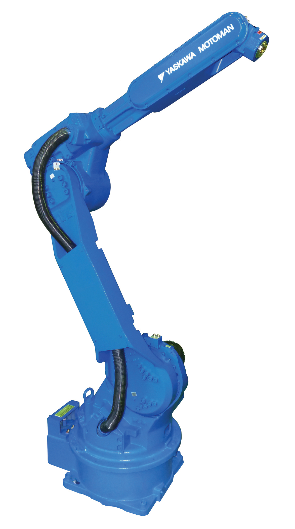

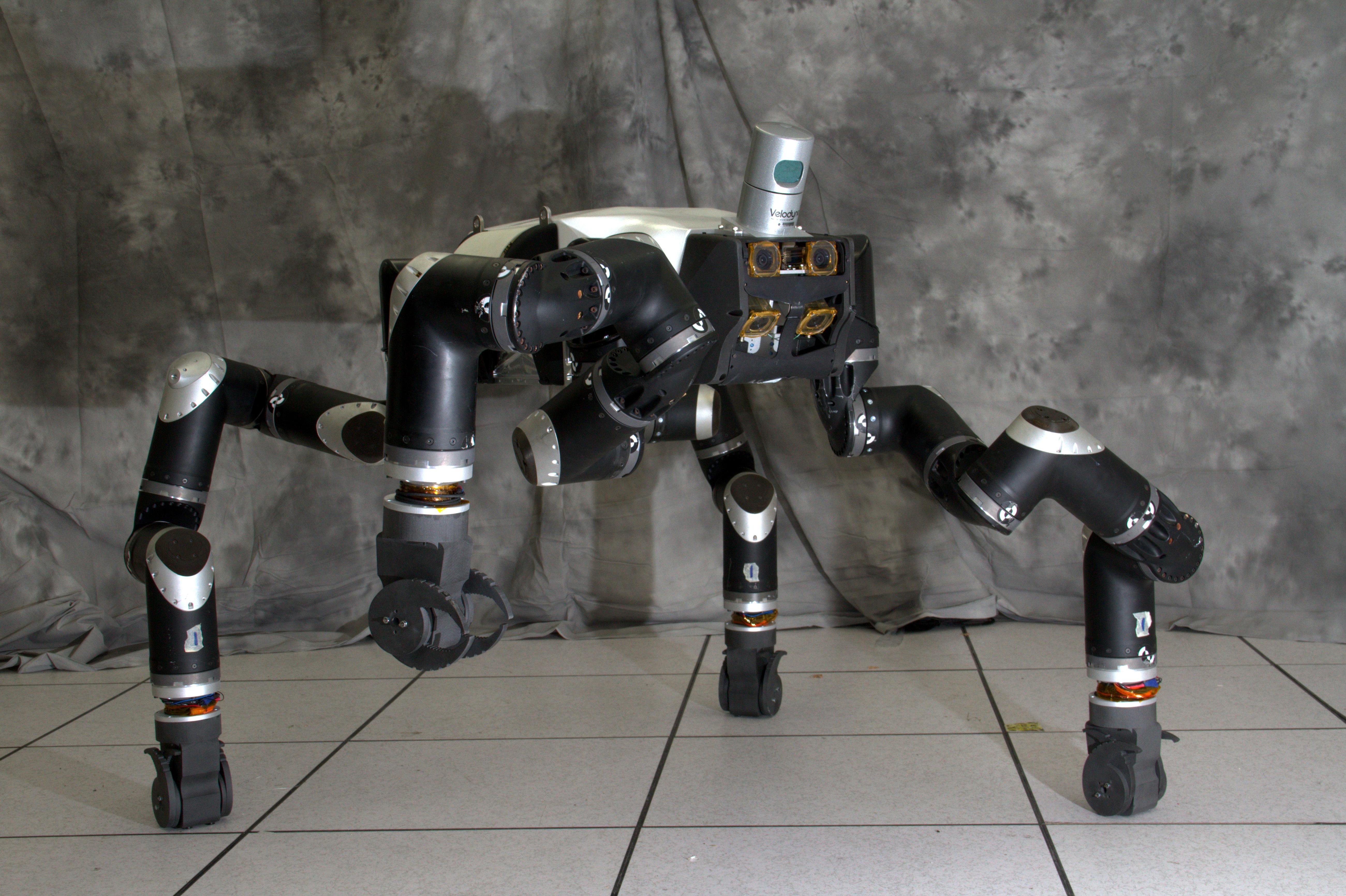


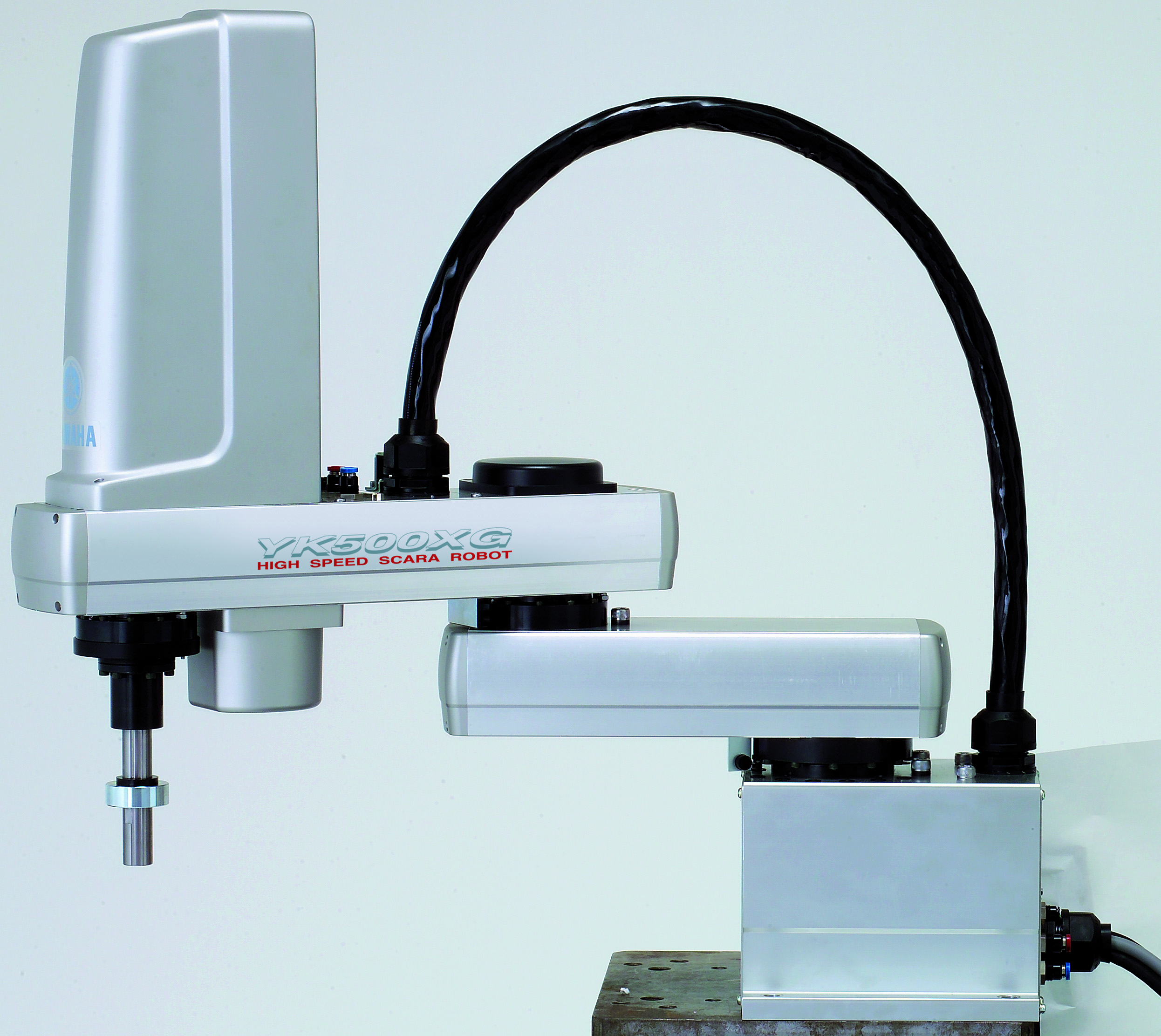
![Figure 3.16: Vertical view of a SCARA robot, with end-effector location (x,y). In the triangle (p_0,p_1,p_2), define \gamma\in[0,\pi] as the angle opposite the side \segment{p_0p_2}](figures/robot-2link-inversekinematics.svg)